count_ratio <- exp(coef(reg)[-1])
conf_int <- exp(confint(reg))[-1, ]
driver_age_vars <- grep("^DrivAge", names(count_ratio), value = TRUE)
data_age <- tibble(
variable = driver_age_vars,
coefficient = count_ratio[driver_age_vars],
lower_bound = conf_int[driver_age_vars, 1],
upper_bound = conf_int[driver_age_vars, 2]
)
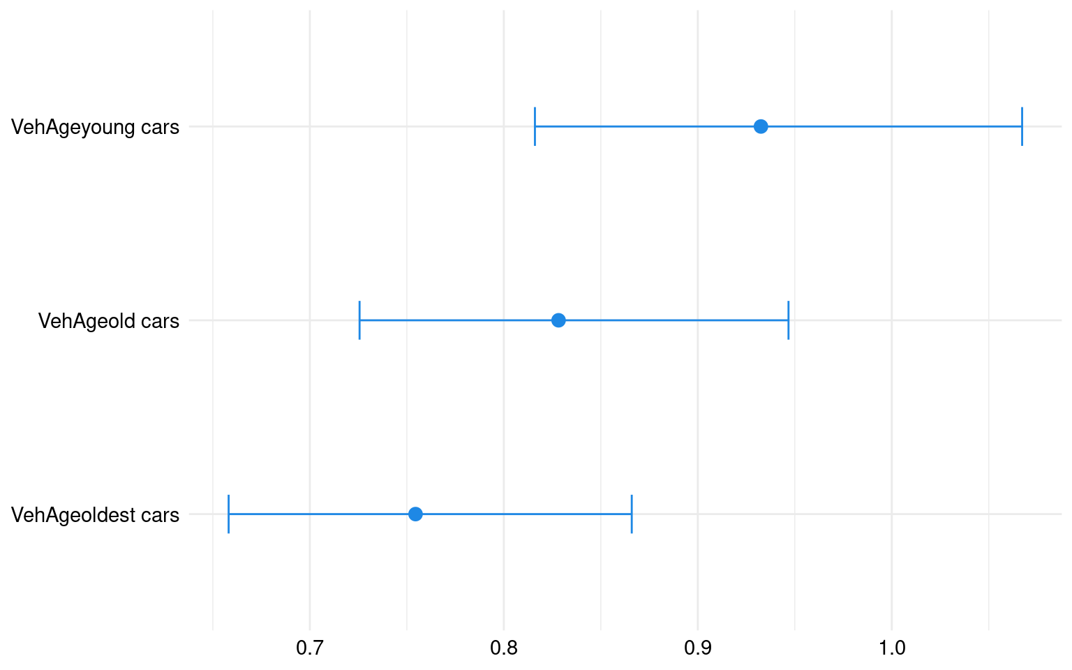
driver_vehage_vars <- grep("^VehAge", names(count_ratio), value = TRUE)
data_vehage <- tibble(
variable = driver_vehage_vars,
coefficient = count_ratio[driver_vehage_vars],
lower_bound = conf_int[driver_vehage_vars, 1],
upper_bound = conf_int[driver_vehage_vars, 2]
)
data_age$variable <- factor(data_age$variable, levels = rev(driver_age_vars))
ggplot(
data_age,
aes(
x = coefficient,
y = variable,
xmin = lower_bound,
xmax = upper_bound
)
) +
geom_point(stat = "identity", size = 3, color = "#1E88E5") +
geom_errorbar(
width = 0.2,
position = position_dodge(width = 0.6),
color = "#1E88E5"
) +
labs(
x = NULL,
y = NULL
) +
global_theme()