Frequency analysis of a French Motor Third Party Liability dataset

Julien Siharath

September, 2024

Introduction

Session Settings

# Graphs----
face_text='plain'
face_title='plain'
size_title = 14
size_text = 11
legend_size = 11

global_theme <- function() {
  theme_minimal() %+replace%
    theme(
      text = element_text(size = size_text, face = face_text),
      legend.position = "bottom",
      legend.direction = "horizontal", 
      legend.box = "vertical",
      legend.key = element_blank(),
      legend.text = element_text(size = legend_size),
      axis.text = element_text(size = size_text, face = face_text), 
      plot.title = element_text(
        size = size_title, 
        hjust = 0.5
      ),
      plot.subtitle = element_text(hjust = 0.5)
    )
}

# Outputs
options("digits" = 2)

In Brief

The objective of this vignette is to demonstrate the application of Poisson regression in analyzing insurance data, specifically focusing on the freMTPLfreq and freMTPLsev datasets from Charpentier (2014). These datasets provide information on insurance contracts and claims related to French motor third-party liability insurance.

By leveraging Poisson regression, our goal is to model the frequency of claims and investigate the factors influencing claim occurrence within the insurance data. Understanding these factors is crucial for accurate risk assessment, pricing strategies, and effective decision-making in the insurance industry.

Required Packages

Show the code

required_libraries <- c(
  "tidyverse", 
  "CASdatasets",
  "glmnet",
  "AER",
  "broom",
  "knitr",
  "kableExtra"
)
invisible(lapply(required_libraries, library, character.only = TRUE))

Data

The Data used in this vignette come from French motor third party liability insurance portfolio.

The first dataset, freMTPLfreq, encompasses details regarding contracts and clients obtained from a French insurance company, related to some motor insurance portfolio.

The second dataset, freMTPLsev, contains claims information, from the same company.

For convenience, the freMTPLfreq table will be named CONTRACTS hereafter. The freMTPLsev will be named CLAIMS

Dictionaries

The list of the 10 variables from the freMTPLfreq dataset is reported in Table 1. Similarly, the two variables encapsulated within the freMTPLsev dataset are reported in table Table 2.

Table 1: Content of the freMTPLfreq dataset: CONTRACTS

Attribute	Type	Description
PolicyID	Numeric	Unique identifier for the contract
ClaimNB	Numeric	Number of claims during the exposure period
Exposure	Numeric	Exposure duration in years
Power	Factor	Power of the car (ordered categorical)
CarAge	Numeric	Age of the car in years
DriverAge	Numeric	Age of the driver in years
Brand	Factor	Brand of the car categorized
Gaz	Factor	Type of fuel used (diesel or regular)
Region	Factor	Region in France where the driver resides
Density	Numeric	Population density in the city where the driver resides

Table 2: Content of the freMTPLsev dataset: CLAIMS

Attribute	Type	Description
PolicyID	Numeric	Unique identifier for the contract
ClaimAmount	Numeric	Cost of the claim, seen as at a recent date

Importation

Code for importing our datasets

data("freMTPLfreq")
data("freMTPLsev")

CONTRACTS <- freMTPLfreq |>
  filter(Exposure > 0.90)


# Create factors
CONTRACTS.f <- 
  CONTRACTS |> 
  mutate(
    DriverAge = cut(DriverAge, c(17, 22, 26, 42, 74, Inf)),
    CarAge = cut(CarAge, c(0, 1, 4, 15, Inf), include.lowest = TRUE),
    Density = cut(Density, c(0, 40, 200, 500, 4500, Inf), include.lowest = TRUE)
  )


CLAIMS <- freMTPLsev |>
  as_tibble()

# check
if (sum(freMTPLsev$PolicyID %in% CONTRACTS$PolicyID) == sum(CONTRACTS$ClaimNb)) {
  message("Data import has been completed successfully.")
} else {
  stop("Error when importing data: numbers are not equal.")
}

Models

Purpose

In the realm of automobile insurance, Poisson regression is a reliable tool for understanding and predicting accident frequencies, repair costs, and claims trends.

By utilizing Poisson regression, insurers can anticipate forthcoming challenges, refine pricing strategies, and ensure resilience in a dynamic landscape of risk.

Pay Attention

The results from Poisson regression models are valid if:

• the responses are independent.
  
• the responses are distributed according to a Poisson distribution with parameter Lambda.
  
• there is no overdispersion.

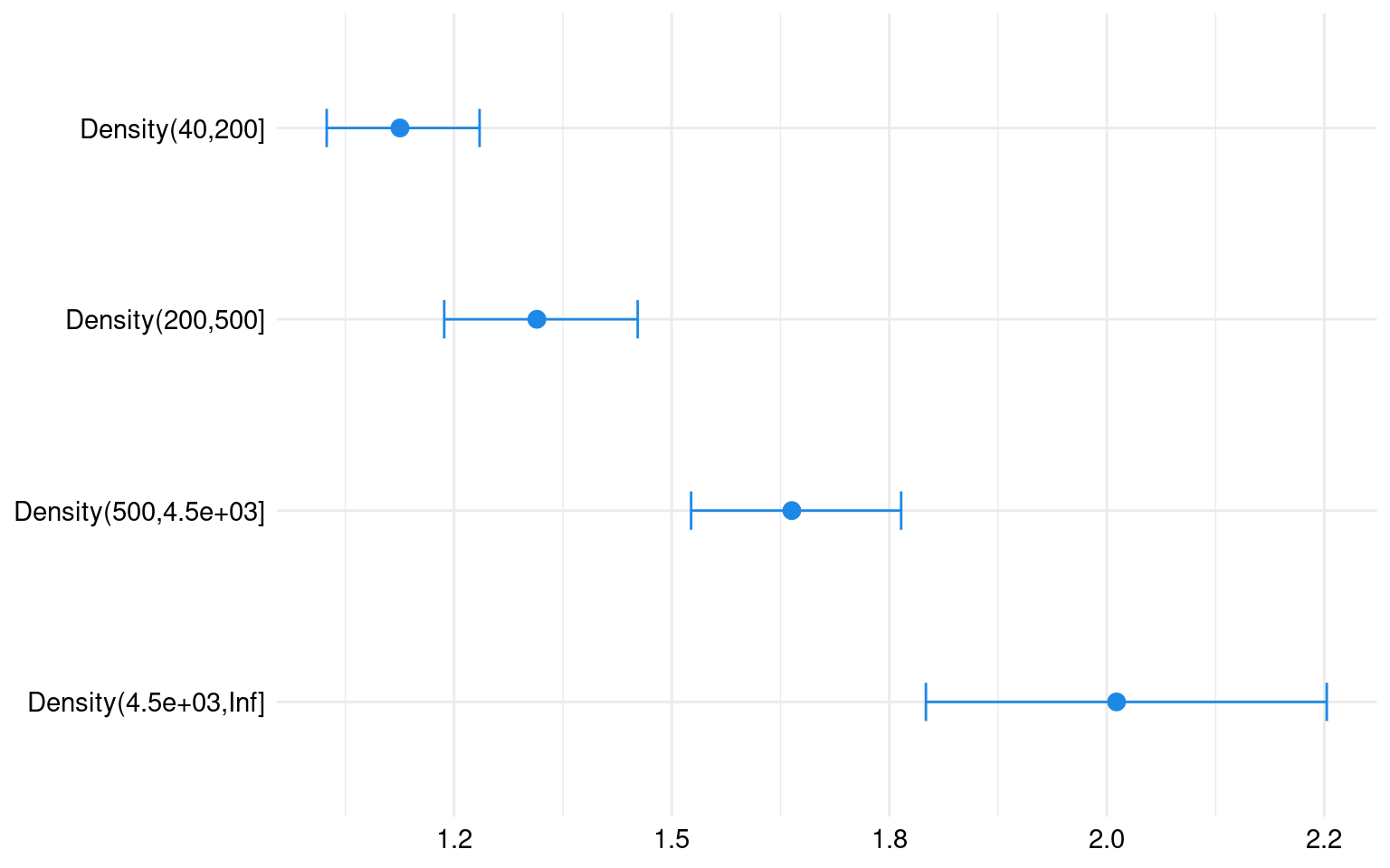
In this analysis, we will explore the relationship between the response variable ClaimNb and the explanatory variables DriverAge and Density. This modeling framework aligns with the principles outlined by Agresti (2013), a prominent figure in statistical methodology, who emphasizes the significance of considering multiple explanatory factors in regression analysis.

To model the frequency of insurance claims, we employ a Poisson regression approach. The response variable in our model, denoted as ClaimNb, represents the count of insurance claims and is assumed to follow a Poisson distribution:

$$\text{ClaimNb} \sim \text{Poisson}(\lambda),$$

where $\lambda$ is the mean rate of claims. The Poisson regression model relates $\lambda$ to a set of predictor variables through a logarithmic link function. This link function ensures that the predicted rate of claims is always positive, as required by the Poisson distribution. More precisely, we express the natural logarithm of $\lambda$ as a linear combination of the predictors:

$$\log{(\lambda)} = \beta_0 + \beta_1 \times \text{DriverAge} + \beta_2 \times \text{Density},$$

where DriverAge represents the age of the driver, Density indicates the population density of the city in which the driver resides, and $\beta_0$, $\beta_1$, and $\beta_2$ are the regression coefficients that need to be estimated.

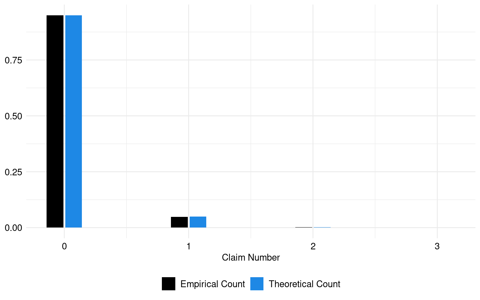
The estimated lambda parameter, which represents the mean of claims, is: 0.05.

set.seed(1234) 

theoretic_count <- rpois(nrow(CONTRACTS.f), mean(CONTRACTS.f$ClaimNb))

tc_df <- tibble(theoretic_count)

freq_theoretic <- prop.table(table(tc_df$theoretic_count))

freq_claim <- prop.table(table(CONTRACTS.f$ClaimNb))

freq_theoretic_df <- tibble(
  Count = as.numeric(names(freq_theoretic)),
  Frequency = as.numeric(freq_theoretic),
  Source = "Theoretical Count"
)

freq_claim_df <- tibble(
  Count = as.numeric(names(freq_claim)),
  Frequency = as.numeric(freq_claim),
  Source = "Empirical Count"
)

freq_combined <- freq_theoretic_df |> 
  rbind(freq_claim_df)

The theoretical and empirical histograms associated with a Poisson distribution are shown in Figure 1.

Code for the following graph

ggplot(freq_combined, aes(x = Count, y = Frequency, fill = Source)) +
  geom_bar(stat = "identity", position = "dodge2", width = 0.3) +
  labs(x = "Claim Number", y = "Frequency", fill = "Legend") +
  theme(legend.position = "right") +
  scale_fill_manual(
    NULL,
    values = c("Empirical Count" = "black", "Theoretical Count" = "#1E88E5")
  ) +
  labs(fill = "Legend") +
  labs(x = "Claim Number", y = NULL) +
  theme(legend.position = "right")+
  global_theme()

Figure 1: Theoretical and empirical histogram of claims in frequence

Model

reg <- glm(
  ClaimNb ~ DriverAge + Density,
  family = poisson,
  data = CONTRACTS.f
)

summary(reg)

Call:
glm(formula = ClaimNb ~ DriverAge + Density, family = poisson,
    data = CONTRACTS.f)

Coefficients:
                     Estimate Std. Error z value Pr(>|z|)
(Intercept)           -2.5436     0.0843  -30.16  < 2e-16 ***
DriverAge(22,26]      -0.3902     0.1009   -3.87  0.00011 ***
DriverAge(26,42]      -0.7148     0.0819   -8.73  < 2e-16 ***
DriverAge(42,74]      -0.7152     0.0807   -8.87  < 2e-16 ***
DriverAge(74,Inf]     -0.6946     0.0924   -7.52  5.5e-14 ***
Density(40,200]        0.1721     0.0377    4.57  4.9e-06 ***
Density(200,500]       0.2965     0.0421    7.04  1.9e-12 ***
Density(500,4.5e+03]   0.4935     0.0375   13.15  < 2e-16 ***
Density(4.5e+03,Inf]   0.6987     0.0583   11.98  < 2e-16 ***
---
Signif. codes:  0 '***' 0.001 '**' 0.01 '*' 0.05 '.' 0.1 ' ' 1

(Dispersion parameter for poisson family taken to be 1)

    Null deviance: 42434  on 135106  degrees of freedom
Residual deviance: 42071  on 135098  degrees of freedom
AIC: 55722

Number of Fisher Scoring iterations: 6

dispersiontest(reg)

    Overdispersion test

data:  reg
z = 7, p-value = 5e-12
alternative hypothesis: true dispersion is greater than 1
sample estimates:
dispersion
         1 

This is a Poisson regression model predicting ClaimNb (number of claims) with DriverAge and Density as predictors. The coefficients in the model indicate the change in the log count of claims associated with each predictor level compared to a reference level.

For example, as DriverAge increases from 22 to 26, the log count of claims decreases by 0.39. Similarly, as Density increases within each category, the log count of claims increases.

All coefficients in the model are statistically significant, reinforcing the reliability of these predictors in explaining the variation in the number of insurance claims.

Presence of overdispersion

Overdispersion can lead to an inadequate model fit, inflated standard errors, incorrect inference, and biased parameter estimates. As such, the following interpretations should be approached with caution. Addressing overdispersion may require alternative modeling approaches, such as negative binomial regression or quasi-Poisson regression, which offer greater flexibility in capturing the variability in the data.

• Coefficients
• Count-Ratio
• Confidence intervals

• Code to create the table

  reg_coef <- tidy(reg)
  
  reg_coef$p.value <- format(reg_coef$p.value, scientific = TRUE, digits = 3)
  
  reg_coef <- reg_coef |>
    mutate(significance = case_when(
      p.value < 0.001 ~ "***",
      p.value < 0.01 ~ "**",
      p.value < 0.05 ~ "*",
      TRUE ~ ""
    ))
  
  kable(reg_coef, format = "html", escape = FALSE) |>
    kable_styling(full_width = FALSE) |>
    add_footnote(c("Significance levels: *** p < 0.001, ** p < 0.01, * p < 0.05"), notation = "none")

  Table 3: Coefficients

  term	estimate	std.error	statistic	p.value	significance
  (Intercept)	-2.54	0.08	-30.2	7.79e-200
  DriverAge(22,26]	-0.39	0.10	-3.9	1.10e-04	***
  DriverAge(26,42]	-0.71	0.08	-8.7	2.64e-18	***
  DriverAge(42,74]	-0.72	0.08	-8.9	7.56e-19	***
  DriverAge(74,Inf]	-0.69	0.09	-7.5	5.46e-14	***
  Density(40,200]	0.17	0.04	4.6	4.92e-06	***
  Density(200,500]	0.30	0.04	7.0	1.91e-12	***
  Density(500,4.5e+03]	0.49	0.04	13.2	1.74e-39	***
  Density(4.5e+03,Inf]	0.70	0.06	12.0	4.65e-33	***
  Significance levels: *** p < 0.001, ** p < 0.01, * p < 0.05

Code to create the table

reg_count_ratio <- tidy(exp(coef(reg)[-1]))

reg_count_ratio <- reg_count_ratio |>
  mutate(p.value = reg_coef$p.value[-1]) |>
  mutate(significance = case_when(
    p.value < 0.001 ~ "***",
    p.value < 0.01 ~ "**",
    p.value < 0.05 ~ "*",
    TRUE ~ ""
  )) |>
  dplyr::select(-p.value)

kable(reg_count_ratio, format = "html", escape = FALSE) |>
  kable_styling(full_width = FALSE) |>
  add_footnote(c("Significance levels: *** p < 0.001, ** p < 0.01, * p < 0.05"), notation = "none")

Table 4: Count Ratio

names	x	significance
DriverAge(22,26]	0.68	***
DriverAge(26,42]	0.49	***
DriverAge(42,74]	0.49	***
DriverAge(74,Inf]	0.50	***
Density(40,200]	1.19	***
Density(200,500]	1.35	***
Density(500,4.5e+03]	1.64	***
Density(4.5e+03,Inf]	2.01	***
Significance levels: *** p < 0.001, ** p < 0.01, * p < 0.05

Each count ratio represents the change in the count of making a claim associated with a one-unit increase in the predictor variable, compared to the reference category DriverAge (18,22]. For example, a count ratio of 0.68 for DriverAge (22,26] implies that the count of making a claim for individuals aged 22 to 26 is approximately 32% lower compared to the reference category.

Similarly, count ratios above 1 for Density categories suggest an increase in the count of making a claim as the population density increases within each category.

Code to create the table

reg_conf_int <- as.data.frame(exp(confint(reg))[-1, ])

Waiting for profiling to be done...

Code to create the table

colnames(reg_conf_int) <- c("2.5 %", "97.5 %")

reg_conf_int <- reg_conf_int |>
  mutate(p.value = reg_coef$p.value[-1]) |>
  mutate(significance = case_when(
    p.value < 0.001 ~ "***",
    p.value < 0.01 ~ "**",
    p.value < 0.05 ~ "*",
    TRUE ~ ""
  )) |>
  dplyr::select(-p.value)

kable(reg_conf_int, format = "html", escape = FALSE) |>
  kable_styling(full_width = FALSE) |>
  add_footnote(c("Significance levels : *** p < 0.001, ** p < 0.01, * p < 0.05"), notation = "none")

Table 5: Confidence intervals

	2.5 %	97.5 %	significance
DriverAge(22,26]	0.56	0.83	***
DriverAge(26,42]	0.42	0.58	***
DriverAge(42,74]	0.42	0.58	***
DriverAge(74,Inf]	0.42	0.60	***
Density(40,200]	1.10	1.28	***
Density(200,500]	1.24	1.46	***
Density(500,4.5e+03]	1.52	1.76	***
Density(4.5e+03,Inf]	1.79	2.25	***
Significance levels : *** p < 0.001, ** p < 0.01, * p < 0.05

Graphs

• DriverAge
• Density

• Code to create the following graph

  count_ratio <- exp(coef(reg)[-1])
  conf_int <- exp(confint(reg))[-1, ]
  
  driver_age_vars <- grep("^DriverAge", names(count_ratio), value = TRUE)
  
  data_age <- tibble(
    variable = driver_age_vars,
    coefficient = count_ratio[driver_age_vars], 
    lower_bound = conf_int[driver_age_vars, 1], 
    upper_bound = conf_int[driver_age_vars, 2]
  )
  
  
  driver_density_vars <- grep("^Density", names(count_ratio), value = TRUE)
  
  data_density <- tibble(
    variable = driver_density_vars,
    coefficient = count_ratio[driver_density_vars], 
    lower_bound = conf_int[driver_density_vars, 1], 
    upper_bound = conf_int[driver_density_vars, 2]
  )
  
  ggplot(
    data_age |>
    mutate(variable = fct_rev(variable)), 
    aes(
      x = coefficient,
      y = variable,
      xmin = lower_bound,
      xmax = upper_bound
    )
  ) +
    geom_point(stat = "identity", size = 3, color = "#1E88E5") +
    geom_errorbar(
      width = 0.2,
      position = position_dodge(width = 0.6),
      color = "#1E88E5"
    ) +
    labs(
      x = NULL,
      y = NULL
    ) +
    global_theme()

  Figure 2: Count ratio and confidence interval of DriverAge

  

Code to create the following graph

data_density <- data_density |> 
  mutate(variable = reorder(variable, coefficient, decreasing = TRUE))

ggplot(
  data_density, 
  aes(
    x = coefficient,
    y = variable,
    xmin = lower_bound,
    xmax = upper_bound
  )
) +
  geom_point(
    stat = "identity",
    size = 3,
    color = "#1E88E5"
  ) +
  geom_errorbar(
    width = 0.2,
    position = position_dodge(width = 0.6),
    color = "#1E88E5"
  ) +
  labs(
    x = NULL,
    y = NULL
  ) +
  global_theme()

Figure 3: count ratio and confidence interval of Density

References

Agresti, Alan. 2013. Categorical Data Analysis, 3rd Edition.

Charpentier, Arthur. 2014. Computational Actuarial Science with R. The R Series. Chapman; Hall/CRC. https://www.routledge.com/Computational-Actuarial-Science-with-R/Charpentier/p/book/9781138033788.

See also

For more similar claim frequency datasets with a Poisson-like distribution, see ausprivauto0405 (import with data("ausprivauto0405")): Australian automobile dataset, norauto: Norwegian automobile dataset (import with data("norauto")), beMTPL16: Belgian automobile dataset (import with data("beMTPL16")), or pg17trainpol (import with data("pg17trainpol")).