Frequency analysis of a Norwegian Motor Third Party Liability dataset

Siharath Julien

2024-09-01

Introduction

Session Settings

# Graphs----
face_text='plain'
face_title='plain'
size_title = 14
size_text = 11
legend_size = 11

global_theme <- function() {
  theme_minimal() %+replace%
    theme(
      text = element_text(size = size_text, face = face_text),
      legend.position = "bottom",
      legend.direction = "horizontal", 
      legend.box = "vertical",
      legend.key = element_blank(),
      legend.text = element_text(size = legend_size),
      axis.text = element_text(size = size_text, face = face_text), 
      plot.title = element_text(
        size = size_title, 
        hjust = 0.5
      ),
      plot.subtitle = element_text(hjust = 0.5)
    )
}

# Outputs
options("digits" = 2)

In Brief

In some instances, zeros appear in the data. A simple Poisson model overlooks this specific structure, leading to inaccurate estimates. To resolve this issue, we employ zero-inflated regression models.

The purpose of this vignette is to demonstrate the application of zero-inflated regression in analyzing insurance data, with a particular focus on the norauto dataset from Charpentier (2014). This dataset contains information on insurance contracts and claims related to Norwegian motor third-party liability insurance. By using zero-inflated regression, we aim to model the frequency of claims and explore the factors influencing claim occurrences within the insurance data.

Required Packages

Show the code

required_libraries <- c(
  "tidyverse", 
  "CASdatasets",
  "pscl",
  "AER",
  "broom",
  "knitr",
  "kableExtra"
)
invisible(lapply(required_libraries, library, character.only = TRUE))

Data

The data used in this vignette come from the motor third-party liability insurance portfolio of a Norwegian insurer, norauto.

The norauto dataset, encompasses details regarding contracts and clients obtained from a Norwegian insurance company, related to a motor insurance portfolio. Third-party insurance insures vehicle owners against injury caused to other drivers, passengers, or pedestrians as a result of an accident.

For convenience, the norauto table will be named CLAIMS.

Dictionaries

The list of the 9 variables from the freMTPLfreq dataset is reported in Table 1.

Table 1: Content of the CLAIMS dataset: norauto

Attribute	Type	Description
Male	Factor	1 if the policyholder is a male, 0 otherwise
Young	Factor	1 if the policyholder age is below 26 years, 0 otherwise
DistLimit	Factor	The distance limit as stated in the insurance contract: “8000 km”, “12000 km”, “16000 km”, “20000 km”, “25000-30000 km”, “no limit”
GeoRegion	Factor	Density of the geographical region (from heaviest to lightest): “High+”, “High-”, “Medium+”, “Medium-”, “Low+”, “Low-”
Expo	Numeric	Exposure as a fraction of year
ClaimAmount	Numeric	0 or the average CLAIMS amount if NbClaim > 0
NbClaim	Numeric	The CLAIMS number

Importation

code for importing our datasets

data(norauto)

CLAIMS <- norauto |>
  filter(Expo > 0.80)

CLAIMS <- 
  CLAIMS |> 
  mutate(
    DistLimit = factor(
      DistLimit,
      levels = c(
        "8000 km", "12000 km", "16000 km", "20000 km", 
        "25000-30000 km", "no limit"
      )
    ),
    GeoRegion = factor(
      GeoRegion,
      levels = c("Low-" , "Low+", "Medium-", "Medium+", "High-", "High+")
    )
  )

Models

Purpose

Zero-inflated regression models offer distinct advantages over simple Poisson regression because they explicitly address zero inflation in the data. Zero-inflated models, such as Zero-inflated Poisson (ZIP) or Zero-inflated negative binomial (ZINB) regression, recognize that zeros can arise from two distinct processes: structural reasons (e.g., policyholders who never file claims) and random chance.

By incorporating these dual processes, zero-inflated regression models provide more accurate estimates and better predictions, particularly in scenarios where excess zeros are prevalent. This enhances the precision of risk assessments, improves the effectiveness of pricing strategies, and facilitates better decision-making for insurers operating in domains like automobile insurance. These models excel in handling situations characterized by an abundance of zeros in the response variable, making them highly valuable in fields such as insurance claims analysis, healthcare data analytics, and ecological studies.

Pay Attention

The results from Zero-inflated regression models are valid if:

• the responses are independent.
  
• the responses are distributed according to a Poisson distribution with parameter Lambda.
  
• There may be overdispersion present in the data.

In this analysis, we will explore the relationship between the response variable NbClaim and the explanatory variables Young, Male, DistLimit and GeoRegion. This modeling framework aligns with the principles outlined by Agresti (2013), a prominent figure in statistical methodology, who emphasizes the significance of considering multiple explanatory factors in regression analysis.

To model the frequency of insurance claims, we employ a Zero-Inflated Negative Binomial (ZINB) Regression approach for the response variable NbClaim, which represents the count of insurance claims and is assumed to follow a Negative Binomial distribution:

$$\text{NbClaim} \sim \text{NegBin}(\mu, \theta),$$ where $\mu$ is the mean rate of claims and $\theta$ is the dispersion parameter that controls the variance of the distribution. The ZINB approach allows for flexible, nonlinear relationships and accounts for excess zeros in the data. More precisely, we express the natural logarithm of $\mu$ as a combination of predictor variables and an additional term accounting for exposure:

$$\log(\mu) = \beta_0 + \beta_1 \times \text{Young} + \beta_2 \times \text{Male} + \beta_3 \times \text{DistLimit} + \beta_4 \times \text{GeoRegion} + \text{log(Exposure)},$$ where Young is a variable indicating if the driver is young, Male is a variable indicating if the driver is male, DistLimit represents the distance limit on the insurance policy, GeoRegion denotes the density of the geographical region, $\ \log(\text{Exposure})$ adjusts for the exposure variable and $\beta_0,\ \beta_1,\ \beta_2,\ \beta_3,\ \beta_4$ are the coefficients to be estimated.

Additionally, the zero-inflation component models the probability of excess zeros using a logistic regression: $$\text{Logit}(P(\text{zero})) = Z\gamma$$ where $Z$ represents the matrices of covariates for the or the zero-inflation model and $\gamma$ are the vectors of coefficients.

In this model, the intercept $\beta_0$ and the coefficients $\beta_0,\ \beta_1,\ \beta_2,\ \beta_3,\ \beta_4$ are estimated through regression to quantify their impact on the expected rate of claims. The logistic regression for zero inflation allows the model to capture complex, nonlinear relationships and the presence of excess zeros in the data, providing a more flexible and accurate fit.

The estimated $\mu$ parameter, which represents the mean of claims, is 0.08.

set.seed(1234) 

theoretic_count <- rpois(nrow(CLAIMS), mean(CLAIMS$NbClaim))

tc_df <- tibble(theoretic_count)

freq_theoretic <- prop.table(table(tc_df$theoretic_count))

freq_claim <- prop.table(table(CLAIMS$NbClaim))

freq_theoretic_df <- tibble(
  Count = as.numeric(names(freq_theoretic)),
  Frequency = as.numeric(freq_theoretic),
  Source = "Theoretical Count"
)

freq_claim_df <- tibble(
  Count = as.numeric(names(freq_claim)),
  Frequency = as.numeric(freq_claim),
  Source = "Empirical Count"
)

freq_combined <- freq_theoretic_df |> 
  rbind(freq_claim_df)

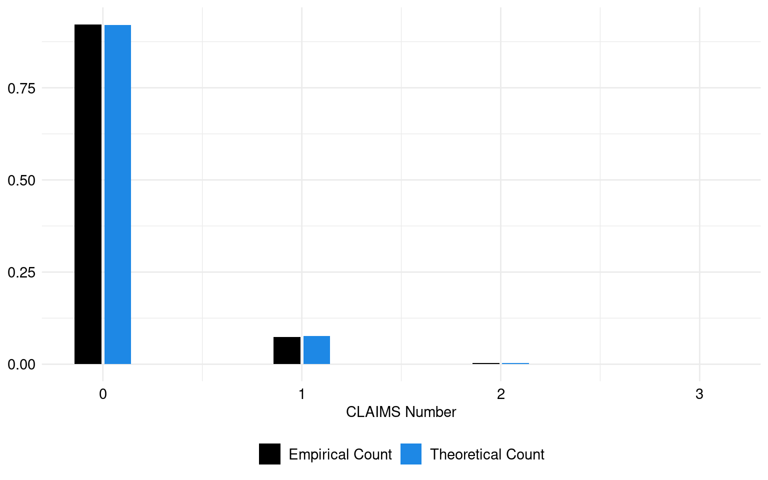
The theoretical and empirical histograms associated with a Poisson distribution are shown in Figure 1.

Code for the following graph

ggplot(freq_combined, aes(x = Count, y = Frequency, fill = Source)) +
  geom_bar(stat = "identity", position = "dodge2", width = 0.3) +
  labs(x = "CLAIMS Number", y = "Frequency", fill = "Legend") +
  theme(legend.position = "right") +
  scale_fill_manual(
    NULL,
    values = c("Empirical Count" = "black", "Theoretical Count" = "#1E88E5")
  ) +
  labs(fill = "Legend") +
  labs(x = "CLAIMS Number", y = NULL) +
  theme(legend.position = "right")+
  global_theme()

Figure 1: Theoretical and empirical histogram of claims in frequence

freg <- formula(NbClaim ~ Young + Male + DistLimit + GeoRegion + offset(log(Expo)) | Young + Male + DistLimit + GeoRegion)

reg <- zeroinfl(freg, data = CLAIMS, dist = "negbin")

summary(reg)

Call:
zeroinfl(formula = freg, data = CLAIMS, dist = "negbin")

Pearson residuals:
   Min     1Q Median     3Q    Max
-0.999 -0.299 -0.264 -0.223 11.753

Count model coefficients (negbin with log link):
                        Estimate Std. Error z value Pr(>|z|)
(Intercept)              -2.4734     0.2770   -8.93  < 2e-16 ***
Young                     0.1483     0.0528    2.81   0.0049 **
Male                     -0.6596     0.1249   -5.28  1.3e-07 ***
DistLimit12000 km         0.0944     0.0824    1.15   0.2519
DistLimit16000 km         0.1929     0.0908    2.13   0.0335 *
DistLimit20000 km         0.4508     0.0761    5.92  3.2e-09 ***
DistLimit25000-30000 km   0.5626     0.0732    7.69  1.5e-14 ***
DistLimitno limit         0.7454     0.0682   10.94  < 2e-16 ***
GeoRegionLow+            -0.1212     0.3054   -0.40   0.6915
GeoRegionMedium-         -0.0910     0.2429   -0.37   0.7080
GeoRegionMedium+          0.0708     0.2286    0.31   0.7569
GeoRegionHigh-           -0.0283     0.2397   -0.12   0.9061
GeoRegionHigh+            0.2103     0.2363    0.89   0.3736
Log(theta)               10.2954    54.3029    0.19   0.8496

Zero-inflation model coefficients (binomial with logit link):
                        Estimate Std. Error z value Pr(>|z|)
(Intercept)                0.618      1.435    0.43   0.6669
Young                      1.685      0.903    1.87   0.0620 .
Male                      -2.187      0.750   -2.92   0.0035 **
DistLimit12000 km         -1.260      1.746   -0.72   0.4705
DistLimit16000 km        -17.753   2531.837   -0.01   0.9944
DistLimit20000 km         -0.031      0.881   -0.04   0.9719
DistLimit25000-30000 km   -0.738      0.920   -0.80   0.4224
DistLimitno limit         -0.706      0.774   -0.91   0.3617
GeoRegionLow+              0.315      1.742    0.18   0.8564
GeoRegionMedium-         -12.684    175.754   -0.07   0.9425
GeoRegionMedium+          -0.521      1.314   -0.40   0.6919
GeoRegionHigh-            -3.876      3.356   -1.15   0.2481
GeoRegionHigh+            -2.660      1.738   -1.53   0.1259
---
Signif. codes:  0 '***' 0.001 '**' 0.01 '*' 0.05 '.' 0.1 ' ' 1

Theta = 29594.892
Number of iterations in BFGS optimization: 111
Log-likelihood: -1.83e+04 on 27 Df

This Zero-Inflated Negative Binomial (ZINB) regression model is used to predict the number of claims (NbClaim) based on the predictors Young, Male, DistLimit, and GeoRegion.

Count Model (Negative Binomial with Log Link)

In the count component, the coefficients reflect the estimated change in the log count of claims associated with each predictor, relative to a reference level. Most of these coefficients are statistically significant (p < 0.05), highlighting their importance in predicting claim counts. For instance, being classified as Young (under 26 years old) or Male influences the expected number of claims.

Zero-Inflation Model (Binomial with Logit Link)

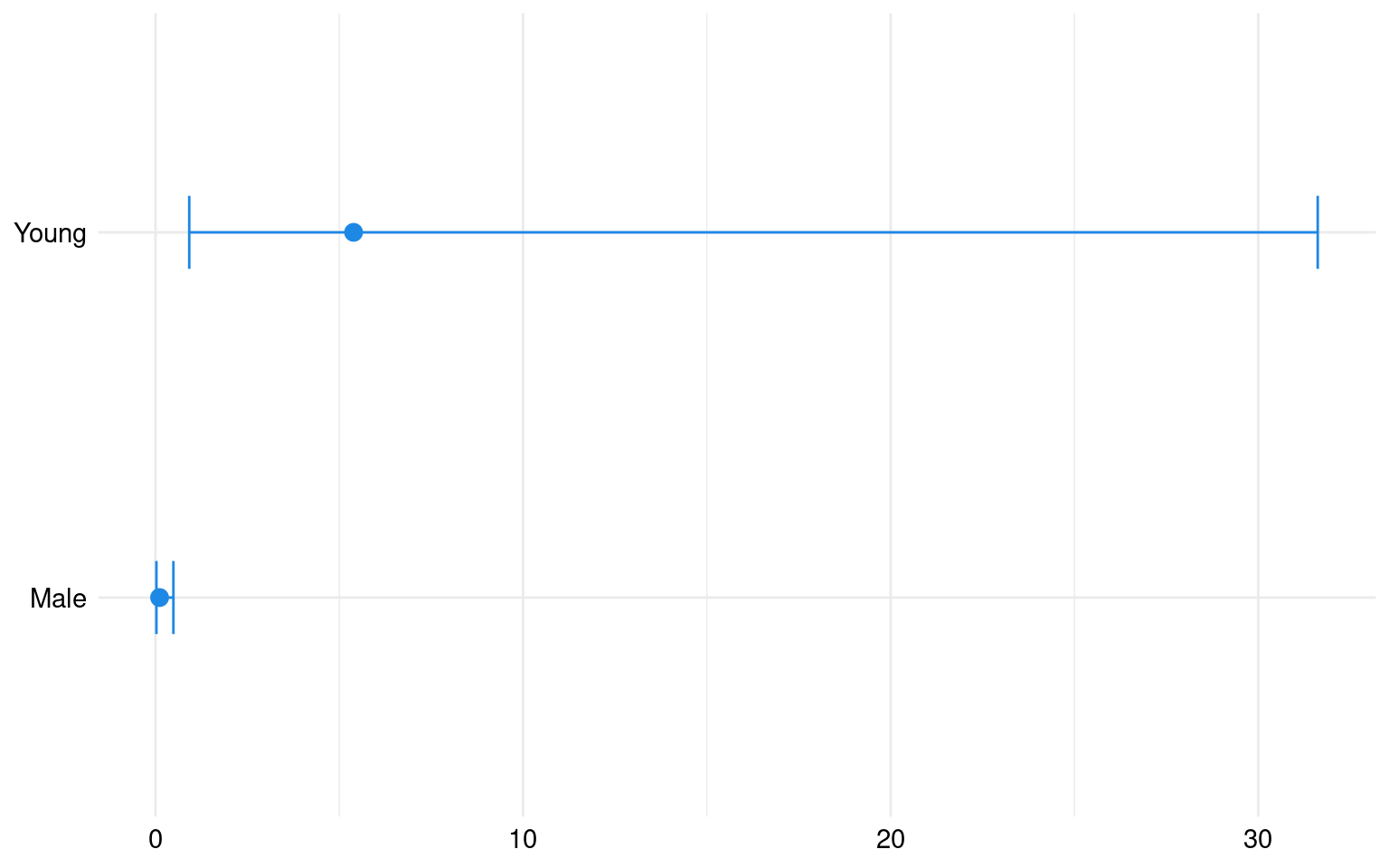
The zero-inflation model coefficients represent the log-odds of excess zeros (instances with no claims) compared to non-excess zeros. Some variables, such as Young and Male, have statistically significant coefficients (p < 0.05), indicating their influence on the likelihood of excess zeros. Specifically:

• If the insured individual is classified as Young (under 26 years old), the log-odds of excess zeros increase by 1.68, suggesting that younger policyholders are more likely to contribute to the excess zeros.

• Conversely, being Male reduces the log-odds of zero-inflation by 2.19, implying that male drivers are less likely to have zero claims.

The impact of DistLimit on zero-inflation varies, though most effects are not statistically significant, indicating a limited role in predicting excess zeros. Similarly, GeoRegion shows a non-significant impact, suggesting that the geographical density of the region does not strongly influence the probability of zero claims.

• Count
• Zero

• • Coefficients
  • Count-Ratio and Confidence intervals

  Code to create the table

  summary_reg <- summary(reg)
  
  # Create a tidy data frame for the count model coefficients
  tidy_count <- summary_reg$coefficients$count |>
    as.data.frame() |>
    mutate(significance = case_when(
      `Pr(>|z|)` < 0.001 ~ "***",
      `Pr(>|z|)` < 0.01 ~ "**",
      `Pr(>|z|)` < 0.05 ~ "*",
      `Pr(>|z|)` < 0.1 ~ ".",
      TRUE ~ ""
    ))
  
  kable(tidy_count, format = "html", escape = FALSE) |>
    kable_styling(full_width = FALSE) |>
    add_footnote(c("Significance levels : *** p < 0.001, ** p < 0.01, * p < 0.05, . p < 0.1"),
                 notation = "none")

  Table 2: Coefficients for the Count model

  	Estimate	Std. Error	z value	Pr(>|z|)	significance
  (Intercept)	-2.47	0.28	-8.93	0.00	***
  Young	0.15	0.05	2.81	0.00	**
  Male	-0.66	0.12	-5.28	0.00	***
  DistLimit12000 km	0.09	0.08	1.15	0.25
  DistLimit16000 km	0.19	0.09	2.13	0.03	*
  DistLimit20000 km	0.45	0.08	5.92	0.00	***
  DistLimit25000-30000 km	0.56	0.07	7.69	0.00	***
  DistLimitno limit	0.75	0.07	10.94	0.00	***
  GeoRegionLow+	-0.12	0.31	-0.40	0.69
  GeoRegionMedium-	-0.09	0.24	-0.37	0.71
  GeoRegionMedium+	0.07	0.23	0.31	0.76
  GeoRegionHigh-	-0.03	0.24	-0.12	0.91
  GeoRegionHigh+	0.21	0.24	0.89	0.37
  Log(theta)	10.30	54.30	0.19	0.85
  Significance levels : *** p < 0.001, ** p < 0.01, * p < 0.05, . p < 0.1

  Code to create the table

  estimates <- summary_reg$coefficients$count[-1, ] 
  
  exp_estimates <- exp(estimates[, "Estimate"])
  
  p_values <- estimates[, "Pr(>|z|)"]
  
  conf_int <- confint(reg)
  
  conf_int_exp <- exp(conf_int)
  
  reg_count_ratio <- data.frame(
    count_ratio = round(exp_estimates, 2),
    `CI 2.5` = conf_int_exp[2:14, 1],
    `CI 97.5` = conf_int_exp[2:14, 2],
    p.value = p_values
  )
  
  reg_count_ratio <- reg_count_ratio |>
    mutate(significance = case_when(
      p.value < 0.001 ~ "***",
      p.value < 0.01 ~ "**",
      p.value < 0.05 ~ "*",
      p.value < 0.1 ~ ".",
      TRUE ~ ""
    )) |>
    dplyr::select(-p.value)
  
  kable(reg_count_ratio, format = "html", escape = FALSE, digits = 2) |>
    kable_styling(full_width = FALSE) |>
    add_footnote(c("Significance levels: *** p < 0.001, ** p < 0.01, * p < 0.05, . p < 0.1"),
                 notation = "none")

  Table 3: Count Ratio and confidence intervals for the Count model

  	count_ratio	CI.2.5	CI.97.5	significance
  Young	1.2e+00	1.05	1.29	**
  Male	5.2e-01	0.40	0.66	***
  DistLimit12000 km	1.1e+00	0.94	1.29
  DistLimit16000 km	1.2e+00	1.02	1.45	*
  DistLimit20000 km	1.6e+00	1.35	1.82	***
  DistLimit25000-30000 km	1.8e+00	1.52	2.03	***
  DistLimitno limit	2.1e+00	1.84	2.41	***
  GeoRegionLow+	8.9e-01	0.49	1.61
  GeoRegionMedium-	9.1e-01	0.57	1.47
  GeoRegionMedium+	1.1e+00	0.69	1.68
  GeoRegionHigh-	9.7e-01	0.61	1.56
  GeoRegionHigh+	1.2e+00	0.78	1.96
  Log(theta)	3.0e+04	0.11	30.90
  Significance levels: *** p < 0.001, ** p < 0.01, * p < 0.05, . p < 0.1

  Each count ratio represents the change in odds of making a claim associated with a one-unit increase in the predictor variable, relative to the reference category. For instance, a count ratio of 1.16 for Young implies that the odds of making a claim for younger individuals are approximately 16% higher compared to the reference category, which is older individuals. Similarly, a count ratio above 1 for Distlimit categories suggests an increase in the odds of making a claim as the distance limit increases within each category.

• Coefficents
• Count-Ratio and Confidence intervals

code to create the table

# Create a tidy data frame for the zero-inflation model coefficients
tidy_zero <- summary_reg$coefficients$zero |>
  as.data.frame() |>
  mutate(significance = case_when(
    `Pr(>|z|)` < 0.001 ~ "***",
    `Pr(>|z|)` < 0.01 ~ "**",
    `Pr(>|z|)` < 0.05 ~ "*",
    TRUE ~ ""
  ))

kable(tidy_zero, format = "html", escape = FALSE) |>
  kable_styling(full_width = FALSE) |>
  add_footnote(c("Significance levels : *** p < 0.001, ** p < 0.01, * p < 0.05"),
               notation = "none")

Table 4: Coefficients for the Zero model

	Estimate	Std. Error	z value	Pr(>|z|)	significance
(Intercept)	0.62	1.44	0.43	0.67
Young	1.68	0.90	1.87	0.06
Male	-2.19	0.75	-2.92	0.00	**
DistLimit12000 km	-1.26	1.75	-0.72	0.47
DistLimit16000 km	-17.75	2531.84	-0.01	0.99
DistLimit20000 km	-0.03	0.88	-0.04	0.97
DistLimit25000-30000 km	-0.74	0.92	-0.80	0.42
DistLimitno limit	-0.71	0.77	-0.91	0.36
GeoRegionLow+	0.32	1.74	0.18	0.86
GeoRegionMedium-	-12.68	175.75	-0.07	0.94
GeoRegionMedium+	-0.52	1.31	-0.40	0.69
GeoRegionHigh-	-3.88	3.36	-1.15	0.25
GeoRegionHigh+	-2.66	1.74	-1.53	0.13
Significance levels : *** p < 0.001, ** p < 0.01, * p < 0.05

Code to create the table

estimates <- summary_reg$coefficients$zero[-1, ]

exp_estimates <- exp(estimates[, "Estimate"])

p_values <- estimates[, "Pr(>|z|)"]

conf_int <- confint(reg)

conf_int_exp <- exp(conf_int)

reg_count_ratio <- data.frame(
  count_ratio = exp_estimates,
  `CI 2.5` = conf_int_exp[15:26, 1],
  `CI 97.5` = conf_int_exp[15:26, 2],
  p.value = p_values
)

reg_count_ratio <- reg_count_ratio |>
  mutate(significance = case_when(
    p.value < 0.001 ~ "***",
    p.value < 0.01 ~ "**",
    p.value < 0.05 ~ "*",
    p.value < 0.1 ~ ".",
    TRUE ~ ""
  )) |>
  dplyr::select(-p.value)

kable(reg_count_ratio, format = "html", escape = FALSE) |>
  kable_styling(full_width = FALSE) |>
  add_footnote(c("Significance levels: *** p < 0.001, ** p < 0.01, * p < 0.05, . p < 0.1"),
               notation = "none")

Table 5: Count-Ratio and Confidence intervals for the Zero model

	count_ratio	CI.2.5	CI.97.5	significance
Young	5.39	0.92	3.2e+01	.
Male	0.11	0.03	4.9e-01	**
DistLimit12000 km	0.28	0.01	8.7e+00
DistLimit16000 km	0.00	0.00	Inf
DistLimit20000 km	0.97	0.17	5.5e+00
DistLimit25000-30000 km	0.48	0.08	2.9e+00
DistLimitno limit	0.49	0.11	2.2e+00
GeoRegionLow+	1.37	0.05	4.2e+01
GeoRegionMedium-	0.00	0.00	1.2e+144
GeoRegionMedium+	0.59	0.05	7.8e+00
GeoRegionHigh-	0.02	0.00	1.5e+01
GeoRegionHigh+	0.07	0.00	2.1e+00
Significance levels: *** p < 0.001, ** p < 0.01, * p < 0.05, . p < 0.1

Graphs

• Count Model
• Zero Model

• Code to create the following graph

  estimates <- summary_reg$coefficients$count[-1, ] 
  
  count_ratio <- exp(estimates[, "Estimate"])
  
  conf_int <- exp(confint(reg))[-1, ]
  
  vars_count <- grep("^(Young|Male|DistLimit|GeoRegion)", names(count_ratio), value = TRUE)
  
  vars_count_with_count <- paste0("count_", vars_count)
  
  data_age <- tibble(
    variable = vars_count,
    coefficient = count_ratio[vars_count], 
    lower_bound = conf_int[vars_count_with_count, 1], 
    upper_bound = conf_int[vars_count_with_count, 2]
  )
  
  data_age$variable <- factor(data_age$variable, levels = rev(vars_count))
  
  ggplot(
    data_age, 
    aes(
      x = coefficient,
      y = variable,
      xmin = lower_bound,
      xmax = upper_bound
    )
  ) +
    geom_point(stat = "identity", size = 3, color = "#1E88E5") +
    geom_errorbar(
      width = 0.2,
      position = position_dodge(width = 0.6),
      color = "#1E88E5"
    ) +
    labs(
      x = NULL,
      y = NULL
    ) +
    global_theme()

  Figure 2: Counts ratio and confidence intervals of the count model

  

Code to create the following graph

estimates <- summary_reg$coefficients$zero[-1, ] 

count_ratio <- exp(estimates[, "Estimate"])

conf_int <- exp(confint(reg))[-1, ]

vars_zero <- grep("^(Young|Male)", names(count_ratio), value = TRUE)

vars_zero_with_count <- paste0("zero_", vars_zero)

data_zero <- tibble(
  variable = vars_zero,
  coefficient = count_ratio[vars_zero], 
  lower_bound = conf_int[vars_zero_with_count, 1], 
  upper_bound = conf_int[vars_zero_with_count, 2]
)


ggplot(
  data_zero, 
  aes(
    x = coefficient,
    y = variable,
    xmin = lower_bound,
    xmax = upper_bound
  )
) +
  geom_point(
    stat = "identity",
    size = 3,
    color = "#1E88E5"
  ) +
  geom_errorbar(
    width = 0.2,
    position = position_dodge(width = 0.6),
    color = "#1E88E5"
  ) +
  labs(
    x = NULL,
    y = NULL
  ) +
  global_theme()

Figure 3: Odds ratio and confidence interval of the zero model

References

Agresti, Alan. 2013. Categorical Data Analysis, 3rd Edition.

Charpentier, Arthur. 2014. Computational Actuarial Science with R. The R Series. Chapman; Hall/CRC. https://www.routledge.com/Computational-Actuarial-Science-with-R/Charpentier/p/book/9781138033788.

See also

For more similar claim frequency datasets with a Poisson-like distribution, see freMTPL (import with data("freMTPLfreq")): French automobile dataset, beMTPL16: Belgian automobile dataset (import with data("beMTPL16")), ausprivauto0405 (import with data("ausprivauto0405")): Australian automobile dataset, or pg17trainpol (import with data("pg17trainpol")).