Reserving exercice on reporting delays in AIDS Data

Introduction

Session Settings

# Graphs----
face_text='plain'
face_title='plain'
size_title = 14
size_text = 11
legend_size = 11

In Brief

The reported number of Acquired Immune Deficiency Syndrome (AIDS) cases in England and Wales has recently been significantly underestimated due to substantial reporting delays. To address this issue, we will utilize the Chainladder package, specifically employing the MackChainLadder function.

This analysis is crucial for accurately understanding the progression and impact of AIDS, which is essential for effective resource allocation and public health planning. By applying this method to AIDS reports in England and Wales from July 1983 to December 1992, we aim to adjust for reporting delays, thereby providing a more accurate picture of the epidemic’s evolution during this period.

Required Packages

Show the code

required_libraries <- c(
  "tidyverse", 
  "tidyr",
  "ChainLadder",
  "boot",
  "dplyr"
)
invisible(lapply(required_libraries, library, character.only = TRUE))

Data

The AIDS dataset consists of 570 rows and 6 columns, capturing critical information about AIDS cases in England and Wales. Although all AIDS cases are required to be reported to the Communicable Disease Surveillance Centre, there is often a significant delay between diagnosis and reporting. To accurately estimate the prevalence of AIDS, it is essential to account for cases that have been diagnosed but not yet reported.

This dataset, obtained from Angelis and Gilks (1994) and available in the boot package, records reported AIDS cases from July 1983 through December 1992. The data is organized by both the date of diagnosis and the delay in reporting, allowing for a more comprehensive analysis of the reporting delays and their impact on understanding the true prevalence of AIDS.

Dictionaries

The list of the 6 attributes from the aids dataset is reported in Table 1.

Table 1: Content of the aids

Column Name	Description	Notes
year	The year in which the diagnosis was made.
quarter	The quarter of the year in which the diagnosis was made.	Values range from 1 to 4, representing Q1 to Q4.
delay	The time delay (in months) between diagnosis and reporting.	0 indicates reporting within one month. Longer delays are grouped in 3-month intervals, with the value representing the midpoint of the interval (e.g., 2 means the report was delayed between 1 and 3 months).
dud	An indicator of censoring, where categories have incomplete information.	The recorded number is a lower bound only.
time	The number of quarters from July 1983 until the end of the quarter in which the cases were diagnosed.
y	The number of AIDS cases reported.

Importation and triangle transformation

Code for importing the dataset and transforming it into a triangle

data("aids")

aids_agg <- aids |>
  group_by(year, quarter, delay) |>
  summarise(cases = sum(y), .groups = 'drop') |>
  mutate(year_quarter = paste(year, quarter, sep = "-"))

# Create a data frame in long format
aids_long <- aids_agg |>
  select(year_quarter, delay, cases)

# Reshape the data into a wide format (triangle format)
triangle <- aids_long |>
  pivot_wider(names_from = delay,
              values_from = cases,
              values_fill = list(cases = 0)) |>
  arrange(year_quarter)

# Convert the wide format data frame to a matrix
  triangle_matrix <- as.matrix(triangle |>
  select(-year_quarter))  # Exclude the year_quarter column for matrix conversion

rownames(triangle_matrix) <- triangle$year_quarter

# Triangular shape
n_rows <- nrow(triangle_matrix)
n_cols <- ncol(triangle_matrix)
  
for (i in seq_len(n_cols-1)) {
    triangle_matrix[(n_rows - i + 1):n_rows, i+1] <- NA
}

full_rows <- which(rowSums(is.na(triangle_matrix)) == 0)
full_triangle <- triangle_matrix[full_rows, ]
close_data <- colSums(full_triangle, na.rm = TRUE)

triangle_rows <- which(rowSums(is.na(triangle_matrix)) != 0)

triangle_matrix_final <- rbind(close_data, triangle_matrix[triangle_rows, ])

# Convert matrix to a 'triangle' object for chainladder
triangle_cl <- as.triangle(triangle_matrix_final)

print(triangle_cl)

In this context, a triangle is a table used to display data over time, organized across two dimensions:

Lines as Origin Year: Represents the year when the diagnosis occurred.
Columns as Development Year: Indicates the number of months (+/- 1) that have passed since the origin year.

This table structure is instrumental in tracking and analyzing the progression of data from the time of origin over subsequent months. It allows for a clear visualization of how cases develop and accumulate over time, providing valuable insights for further analysis.

Overview

Purpose

The prediction and monitoring of the acquired immune deficiency syndrome (AIDS) epidemic rely heavily on the availability of reliable and complete data on AIDS diagnoses. However, a significant challenge in this context is the considerable delay that often occurs between the diagnosis of an AIDS case and its subsequent reporting to the epidemic monitoring center. In England and Wales, this reporting process is managed by the Public Health Laboratory Service AIDS Centre at the Communicable Disease Surveillance Centre. To effectively utilize AIDS reports, it is crucial to account for cases that have been diagnosed but have not yet been reported.

To address this issue, we will employ the Mack chain ladder method, a statistical tool originally developed for insurance claims forecasting. The method is particularly well-suited for analyzing right-truncated data, making it an ideal choice for correcting delays in reporting. The Mack chain ladder method enables robust predictions of future case reports by estimating the development pattern of reported cases over time. This approach not only adjusts for the reporting delay but also provides a measure of the uncertainty associated with these estimates.

By applying the Mack chain ladder method, we aim to achieve more accurate and timely insights into the progression of the AIDS epidemic. Enhanced prediction and monitoring capabilities are essential for effective public health planning, resource allocation, and the implementation of timely interventions to control the spread of the disease. While various statistical techniques have been developed to address this inferential challenge, the Mack chain ladder method is distinguished by its reliability and practicality in handling right-truncated data.

Claims development chart
Origin year plot

Code to create the following graph

plot(as.triangle(triangle_cum[-1, -n_cols]), lattice=TRUE)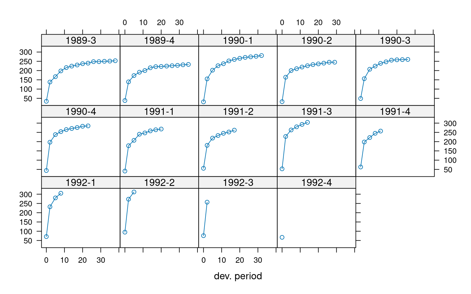

Figure 2: Claims development by origin year

Mack chain-ladder

In 1993, Thomas Mack introduced a groundbreaking method in his paper (Mack 1993), which estimates the standard errors of the chain-ladder forecast without assuming a specific distribution, under three key conditions.

The Mack Chain-Ladder Model

Following the notation established by Mack in 1999 (Mack 1999), let $C_{ik}$ denote the cumulative loss amounts of origin period (e.g., accident year) $i=1,\ldots,m$ , with losses known for development period (e.g., development year) $k \le n+1-i.$

To forecast the amounts $C_{ik}$ for $k > n+1-i$ , the Mack chain-ladder model makes the following assumptions:

$\begin{aligned} \text{CL1:} & \quad E[ F_{ik}| C_{i1},C_{i2},\ldots,C_{ik} ] = f_k \quad \text{where} \quad F_{ik} = \frac{C_{i,k+1}}{C_{ik}} \\ \text{CL2:} & \quad Var\left( \frac{C_{i,k+1}}{C_{ik}} \Bigg| C_{i1},C_{i2}, \ldots,C_{ik} \right) = \frac{\sigma_k^2}{w_{ik} C_{ik}^\alpha} \\ \text{CL3:} & \quad \{C_{i1},\ldots,C_{in}\} \text{ and } \{C_{j1},\ldots,C_{jn}\} \text{ are independent for origin periods } i \neq j \end{aligned}$

where $w_{ik} \in [0,1]$ and $\alpha \in \{0,1,2\}$ are parameters that adjust the variance structure. If these assumptions hold, the Mack chain-ladder model provides an unbiased estimator for Incurred But Not Reported (IBNR) claims.

Intuition Behind the Method

The Chain-Ladder model is a powerful tool used to project future claims based on historical data. The core idea is that claims development patterns are relatively stable and predictable. The model assumes that the ratios of cumulative losses between successive development years are consistent, allowing these ratios to be used in estimating future losses.

Assumptions Explained:

CL1: Expected Future Ratio
This assumption posits that the expected future ratio $F_{ik}$ of cumulative losses between successive development years is constant, given the known losses up to the current development year. Essentially, this means that the ratio of cumulative losses from one development year to the next is assumed to follow a consistent pattern, captured by a factor $f_k$ .
CL2: Variance of Future Ratio
Here, the model specifies that the variance of the future ratio of cumulative losses is proportional to $\frac{\sigma_k^2}{w_{ik} C_{ik}^\alpha}$ . The term $\sigma_k^2$ represents the variability, $w_{ik}$ is a weight, and $\alpha$ is a parameter that adjusts for different variance levels. This assumption is crucial for quantifying the uncertainty around the forecasts.
CL3: Independence of Origin Periods
This assumption ensures that cumulative loss amounts from different origin periods (e.g., different accident years) are independent. This independence simplifies the estimation process and increases the robustness of the model.

Practical Application

The Mack Chain-Ladder model can be viewed as a weighted linear regression through the origin for each development period:

$\text{lm}(y \sim x + 0, \text{weights} = w/x^{2-\alpha}),$

where $y$ is the vector of claims at development period $k+1$ and $x$ is the vector of claims at development period $k$ .

The Mack method is implemented in the ChainLadder package via the function MackChainLadder. This implementation enables actuaries to perform robust reserving exercises, forecast future claims developments, and maintain the financial stability of insurance companies by ensuring they can meet their future claim obligations.

For a comprehensive understanding of this methodology, including its practical implications and applications, see Gesmann (2014).

As an example we apply the MackChainLadder function to our triangle Damage:

mack <- MackChainLadder(triangle_cum, est.sigma="Mack")
mack # same as summary(mack)

MackChainLadder(Triangle = triangle_cum, est.sigma = "Mack")

           Latest Dev.To.Date Ultimate   IBNR Mack.S.E CV(IBNR)
close_data  2,626       1.000    2,626   0.00  0.00000      NaN
1989-3        253       0.980      258   5.21  0.00112 0.000215
1989-4        233       0.972      240   6.67  0.03291 0.004938
1990-1        281       0.969      290   8.99  1.10632 0.123017
1990-2        245       0.960      255  10.08  1.57793 0.156584
1990-3        260       0.949      274  13.88  3.06281 0.220653
1990-4        285       0.935      305  19.94  4.42964 0.222143
1991-1        268       0.918      292  23.97  5.23819 0.218506
1991-2        262       0.896      292  30.45  6.32616 0.207725
1991-3        304       0.867      351  46.59  7.51700 0.161331
1991-4        257       0.829      310  53.12  8.71038 0.163967
1992-1        305       0.783      390  84.52 11.62803 0.137573
1992-2        312       0.708      441 128.97 18.94355 0.146883
1992-3        257       0.584      440 183.05 26.87186 0.146798
1992-4         67       0.153      437 369.56 80.76600 0.218545

            Totals
Latest:   6,215.00
Dev:          0.86
Ultimate: 7,200.02
IBNR:       985.02
Mack.S.E     92.13
CV(IBNR):     0.09

# Displaying the Mack model's parameters
mack$f

 [1] 3.805395 1.211481 1.106679 1.058359 1.046333 1.033174 1.024588 1.018210
 [9] 1.015739 1.011771 1.008844 1.003304 1.007846 1.020599 1.000000

# Viewing the full triangle data from the Mack model
mack$FullTriangle

            dev
origin         0         2         5         8        11        14        17
  close_data 355 1455.0000 1784.0000 2000.0000 2134.0000 2245.0000 2328.0000
  1989-3      34  138.0000  167.0000  198.0000  216.0000  224.0000  230.0000
  1989-4      38  139.0000  173.0000  191.0000  200.0000  215.0000  221.0000
  1990-1      31  155.0000  202.0000  226.0000  237.0000  252.0000  260.0000
  1990-2      32  164.0000  200.0000  210.0000  219.0000  226.0000  232.0000
  1990-3      49  156.0000  207.0000  224.0000  239.0000  247.0000  256.0000
  1990-4      44  197.0000  238.0000  254.0000  265.0000  271.0000  276.0000
  1991-1      41  178.0000  207.0000  240.0000  247.0000  258.0000  264.0000
  1991-2      56  180.0000  219.0000  233.0000  245.0000  252.0000  262.0000
  1991-3      53  228.0000  263.0000  280.0000  293.0000  304.0000  314.0850
  1991-4      63  198.0000  222.0000  245.0000  257.0000  268.9076  277.8284
  1992-1      71  232.0000  280.0000  305.0000  322.7993  337.7556  348.9604
  1992-2      95  273.0000  312.0000  345.2840  365.4343  382.3659  395.0506
  1992-3      76  257.0000  311.3507  344.5654  364.6737  381.5701  394.2284
  1992-4      67  254.9615  308.8810  341.8323  361.7811  378.5435  391.1014
            dev
origin              20        23        26        29        32        35
  close_data 2397.0000 2451.0000 2490.0000 2526.0000 2546.0000 2553.0000
  1989-3      237.0000  240.0000  248.0000  248.0000  250.0000  251.0000
  1989-4      222.0000  224.0000  226.0000  228.0000  231.0000  233.0000
  1990-1      266.0000  271.0000  274.0000  277.0000  281.0000  281.9283
  1990-2      236.0000  240.0000  245.0000  245.0000  247.1668  247.9834
  1990-3      258.0000  259.0000  260.0000  263.0606  265.3871  266.2639
  1990-4      283.0000  285.0000  289.4858  292.8934  295.4838  296.4600
  1991-1      268.0000  272.8802  277.1752  280.4380  282.9182  283.8529
  1991-2      268.4421  273.3304  277.6325  280.9006  283.3849  284.3211
  1991-3      321.8077  327.6678  332.8251  336.7429  339.7212  340.8435
  1991-4      284.6597  289.8432  294.4052  297.8708  300.5052  301.4980
  1992-1      357.5407  364.0514  369.7814  374.1343  377.4432  378.6901
  1992-2      404.7642  412.1348  418.6216  423.5494  427.2954  428.7070
  1992-3      403.9218  411.2771  417.7504  422.6679  426.4061  427.8147
  1992-4      400.7178  408.0148  414.4368  419.3153  423.0238  424.4213
            dev
origin              38        41
  close_data 2573.0000 2626.0000
  1989-3      253.0000  258.2114
  1989-4      234.8281  239.6652
  1990-1      284.1403  289.9932
  1990-2      249.9290  255.0772
  1990-3      268.3530  273.8806
  1990-4      298.7860  304.9405
  1991-1      286.0800  291.9728
  1991-2      286.5519  292.4544
  1991-3      343.5177  350.5936
  1991-4      303.8635  310.1226
  1992-1      381.6613  389.5229
  1992-2      432.0706  440.9706
  1992-3      431.1713  440.0528
  1992-4      427.7513  436.5623

The Mack model factors start at 3.8 for the initial periods and gradually decrease to around 1 in the later periods. These factors represent the development factors for each period, indicating the expected growth in cumulative reports from one period to the next. This trend reflects the typical pattern where most reports occur early in the development process, with the rate of increase diminishing over time.

The triangular data illustrates how reports develop over time for each origin period. For instance, in the 4th quarter of 1992, the number of reported cases of acquired immune deficiency syndrome (AIDS) begins at 67 in the 1st period and grows to 437 cases by the 41st period.

Overall, this output offers a comprehensive view of how reports develop over time and highlights the associated development factors used in the chain ladder method.

References

Angelis, D. De, and W. R. Gilks. 1994. “Estimating Acquired Immune Deficiency Syndrome Accounting for Reporting Delay.” Journal of the Royal Statistical Society, A 157: 31–40.

Gesmann, Markus. 2014. “Claims Reserving and IBNR.” In Computational Actuarial Science with R, 545–84. Chapman; Hall/CRC.

Mack, T. 1993. “Distribution-Free Calculation of the Standard Error of Chain-Ladder Reserve Estimates.” ASTIN Bulletin 23 (2): 213–25.

———. 1999. “The Standard Error of Chain-Ladder Reserve Estimates: Recursive Calculation and Inclusion of a Tail-Factor.” ASTIN Bulletin 29: 361–66.