Session Settings
# Graphs----
face_text='plain'
face_title='plain'
size_title = 14
size_text = 11
legend_size = 11June, 2026
Source:vignettes/triangle_vignette.qmd
# Graphs----
face_text='plain'
face_title='plain'
size_title = 14
size_text = 11
legend_size = 11In Brief
The purpose of this vignette is to illustrate a reserving exercise aimed at forecasting future claims development, with a particular focus on the bottom right corner of the claims triangle and potential further developments. These estimates are crucial for maintaining the financial stability of insurance companies, ensuring that they can meet their future claim obligations.
In this analysis, we will utilize the
fretri1auto9605dataset from Charpentier (2014) and apply techniques from theChainladderpackage to perform the reserving exercise.
The dataset fretri1auto9605 comprises claim triangles for motor policies from a French non-life insurer, spanning the years 1996 to 2005.
In this context, a triangle is a table used to display data over time, structured across two key dimensions:
This table format is instrumental in tracking and analyzing how claims data evolves from the time of origin across subsequent years.
The fretri1auto9605 dataset includes the following elements:
Each of these elements includes two types of triangles:
Paid Claims: These triangles display cumulative claim amounts. For each development year, the amount shown includes all claims paid up to that point. As time progresses, the cumulative total increases or remains the same, reflecting the ongoing addition of payments.
Incurred Claim Amounts: These triangles represent the total estimated amount for claims that have occurred but are not yet fully paid. Unlike paid claims, the incurred amounts are not cumulative. They represent the estimated total cost of claims for a specific development year and can be adjusted based on new information or revisions. Consequently, the incurred amounts may fluctuate over time and do not necessarily follow a simple increasing trend.
In this vignette, we will focus on the triangle representing the paid damage claim amounts, referred to as Damage.
The list of the 3 elements from the fretri1auto9605 dataset is reported in Table 1.
fretri1auto9605
| Elements | Description |
|---|---|
| damage | Represents the damage guarantee for the insurance policy. |
| body | Represents the body guarantee for the insurance policy. |
| total | Represents the total guarantee. |
The list of the 2 triangles in each elements is reported in Table 2.
| Triangle | Description |
|---|---|
| paid | Shows the cumulative amount of claims paid up to each development period. |
| incur | Represents the estimated total amount for claims that have occurred but are not necessarily paid yet. |
data(fretri1auto9605)

Damage <- fretri1auto9605$damage$paid|>
as.triangle()Unlike other industries, the insurance sector sells promises rather than tangible products. An insurance policy represents a commitment by the insurer to cover future claims in exchange for a premium paid upfront.
This unique business model means that insurers do not know the exact cost of their services in advance. Instead, they rely on historical data analysis and expert judgment to set a sustainable price for their offerings. In General Insurance (or Non-Life Insurance, which includes motor, property, and casualty insurance), most policies are valid for a period of 12 months. However, the process of settling claims can extend over several years or even decades. Consequently, insurers often face uncertainty regarding the timing of when claims will be settled.
For example, following a major natural disaster such as an earthquake, the volume of claims can be overwhelming for an insurance company. Assessing the damage to properties, businesses, and personal belongings can be a complex and time-consuming process. Additionally, some claims may require detailed investigations to determine coverage and validate their legitimacy. In such situations, the delay in settlements can be significant, as insurers need time to thoroughly evaluate each claim and ensure accurate payouts.
To forecast future claims and manage pricing effectively, insurers employ methods like chain ladder models. These models are essential tools that estimate future claims based on historical data, helping insurers anticipate upcoming challenges. By using chain ladder models, insurers can provide reliable forecasts, refine pricing strategies, and maintain resilience in a dynamic risk landscape.
In this vignette, we will demonstrate the application of chain ladder models to forecast future claims development using the fretri1auto9605 dataset. This approach will highlight how these models can enhance decision-making in the insurance industry.
For additional insights and a deeper understanding of claims reserving, refer to Gesmann (2014).
ChainLadder::plot(Damage/1000)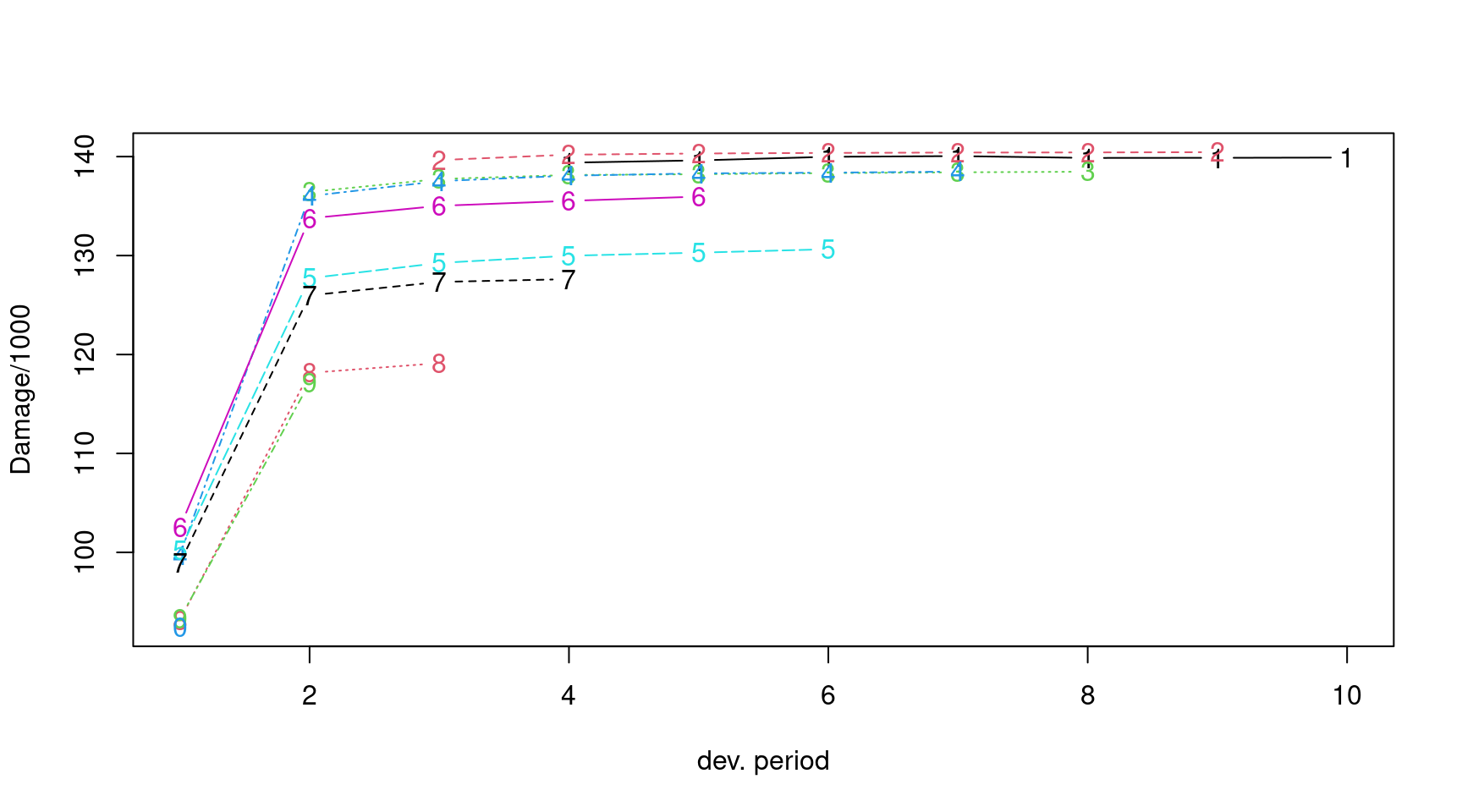
plot(Damage/1000, lattice=TRUE)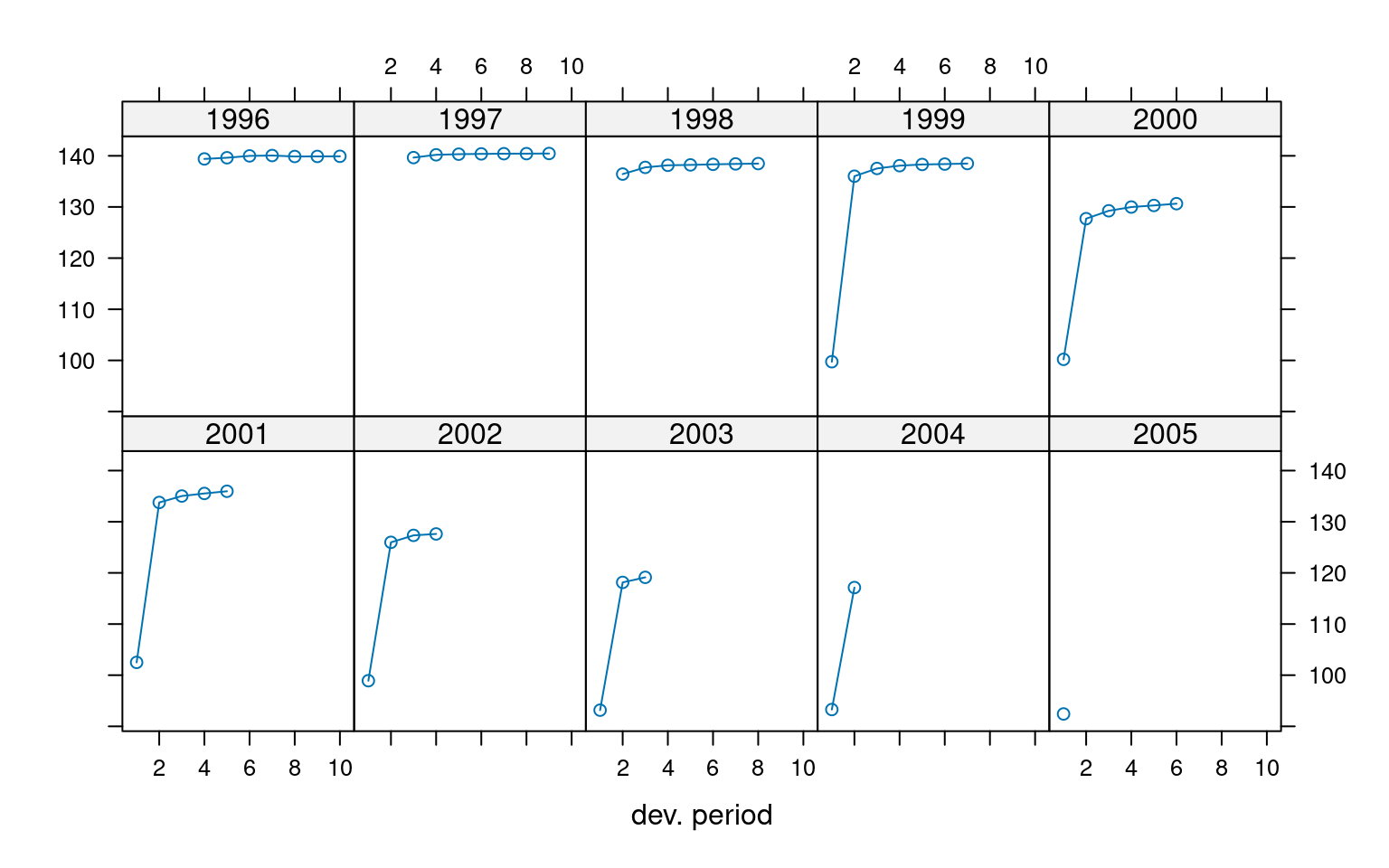
In 1993, Thomas Mack introduced a groundbreaking method in his paper (Mack 1993), which estimates the standard errors of the chain-ladder forecast without assuming a specific distribution, under three key conditions.
Following the notation established by Mack in 1999 (Mack 1999), let denote the cumulative loss amounts of origin period (e.g., accident year) , with losses known for development period (e.g., development year)
To forecast the amounts for , the Mack chain-ladder model makes the following assumptions:
where and are parameters that adjust the variance structure. If these assumptions hold, the Mack chain-ladder model provides an unbiased estimator for Incurred But Not Reported (IBNR) claims.
The Chain-Ladder model is a powerful tool used to project future claims based on historical data. The core idea is that claims development patterns are relatively stable and predictable. The model assumes that the ratios of cumulative losses between successive development years are consistent, allowing these ratios to be used in estimating future losses.
CL1: Expected Future Ratio
This assumption posits that the expected future ratio of cumulative losses between successive development years is constant, given the known losses up to the current development year. Essentially, this means that the ratio of cumulative losses from one development year to the next is assumed to follow a consistent pattern, captured by a factor .
CL2: Variance of Future Ratio
Here, the model specifies that the variance of the future ratio of cumulative losses is proportional to . The term represents the variability, is a weight, and is a parameter that adjusts for different variance levels. This assumption is crucial for quantifying the uncertainty around the forecasts.
CL3: Independence of Origin Periods
This assumption ensures that cumulative loss amounts from different origin periods (e.g., different accident years) are independent. This independence simplifies the estimation process and increases the robustness of the model.
The Mack Chain-Ladder model can be viewed as a weighted linear regression through the origin for each development period:
where is the vector of claims at development period and is the vector of claims at development period .
The Mack method is implemented in the ChainLadder package via the function MackChainLadder. This implementation enables actuaries to perform robust reserving exercises, forecast future claims developments, and maintain the financial stability of insurance companies by ensuring they can meet their future claim obligations.
For a comprehensive understanding of this methodology, including its practical implications and applications, see Gesmann (2014).
As an example we apply the MackChainLadder function to our triangle Damage:
mack <- MackChainLadder(Damage, est.sigma="Mack")
mack # same as summary(mack)
MackChainLadder(Triangle = Damage, est.sigma = "Mack")
Latest Dev.To.Date Ultimate IBNR Mack.S.E CV(IBNR)
1996 139,905 1.000 139,905 0.00 0.00 NaN
1997 140,449 1.000 140,475 26.18 1.06 0.0405
1998 138,476 1.000 138,520 44.15 12.08 0.2736
1999 138,486 1.000 138,494 7.38 150.98 20.4724
2000 130,640 0.999 130,716 76.37 149.00 1.9510
2001 135,956 0.998 136,225 269.20 227.56 0.8453
2002 127,614 0.996 128,084 470.21 258.49 0.5497
2003 119,128 0.993 120,013 885.58 293.16 0.3310
2004 117,133 0.983 119,212 2,079.24 341.87 0.1644
2005 92,422 0.761 121,413 28,991.18 4,143.13 0.1429
Totals
Latest: 1,280,207.64
Dev: 0.97
Ultimate: 1,313,057.12
IBNR: 32,849.48
Mack.S.E 4,227.78
CV(IBNR): 0.13
# Displaying the Mack model's parameters
mack$f
[1] 1.2907697 1.0102412 1.0037355 1.0017012 1.0013946 1.0005313 0.9997345
[8] 1.0001324 1.0001864 1.0000000
# Viewing the full triangle data from the Mack model
mack$FullTriangle
dev
origin 1 2 3 4 5 6 7 8
1996 NA NA NA 139388.2 139619.7 139982.5 140052.8 139867.0
1997 NA NA 139650.2 140195.5 140315.7 140374.0 140411.0 140423.4
1998 NA 136427.9 137736.1 138144.2 138219.5 138330.9 138413.8 138475.9
1999 99741.09 136010.6 137524.4 138070.8 138303.9 138380.3 138486.1 138449.4
2000 100206.10 127709.8 129251.7 129982.1 130291.3 130640.1 130709.5 130674.8
2001 102502.50 133767.4 135024.4 135528.1 135956.1 136145.7 136218.0 136181.9
2002 98919.46 125973.4 127334.7 127613.5 127830.6 128008.9 128076.9 128042.9
2003 93163.87 118141.8 119127.6 119572.6 119776.0 119943.1 120006.8 119974.9
2004 93283.37 117132.5 118332.1 118774.1 118976.2 119142.1 119205.4 119173.8
2005 92422.10 119295.6 120517.4 120967.6 121173.4 121342.3 121406.8 121374.6
dev
origin 9 10
1996 139878.6 139904.6
1997 140449.0 140475.2
1998 138494.2 138520.1
1999 138467.7 138493.5
2000 130692.1 130716.5
2001 136199.9 136225.3
2002 128059.9 128083.7
2003 119990.8 120013.2
2004 119189.6 119211.8
2005 121390.7 121413.3The Mack model development factors begin at approximately 1.3 for the initial periods and gradually decrease to around 1 for the later periods. These factors represent the development factors for each period, indicating the expected growth in cumulative claims from one period to the next. This trend reflects the typical pattern observed in insurance claims, where most claims are reported early in the development process, and the rate of increase diminishes over time as claims stabilize.
The triangular data illustrates how claims evolve over time for each origin period. For instance, considering the origin year 2005, the claims start at 92 422 in the 1st period and increase to 121 413 by the 10th period. This progression is crucial for actuaries when predicting future claims and setting appropriate reserves.
Overall, this output provides a comprehensive view of the claims development process over time and the development factors employed in the chain ladder method. These insights are invaluable for ensuring accurate forecasting and maintaining the financial health of insurance companies.
We can plot the development, including the forecast and estimated standard errors by origin period by setting the argument lattice=TRUE.
plot(mack, lattice=TRUE)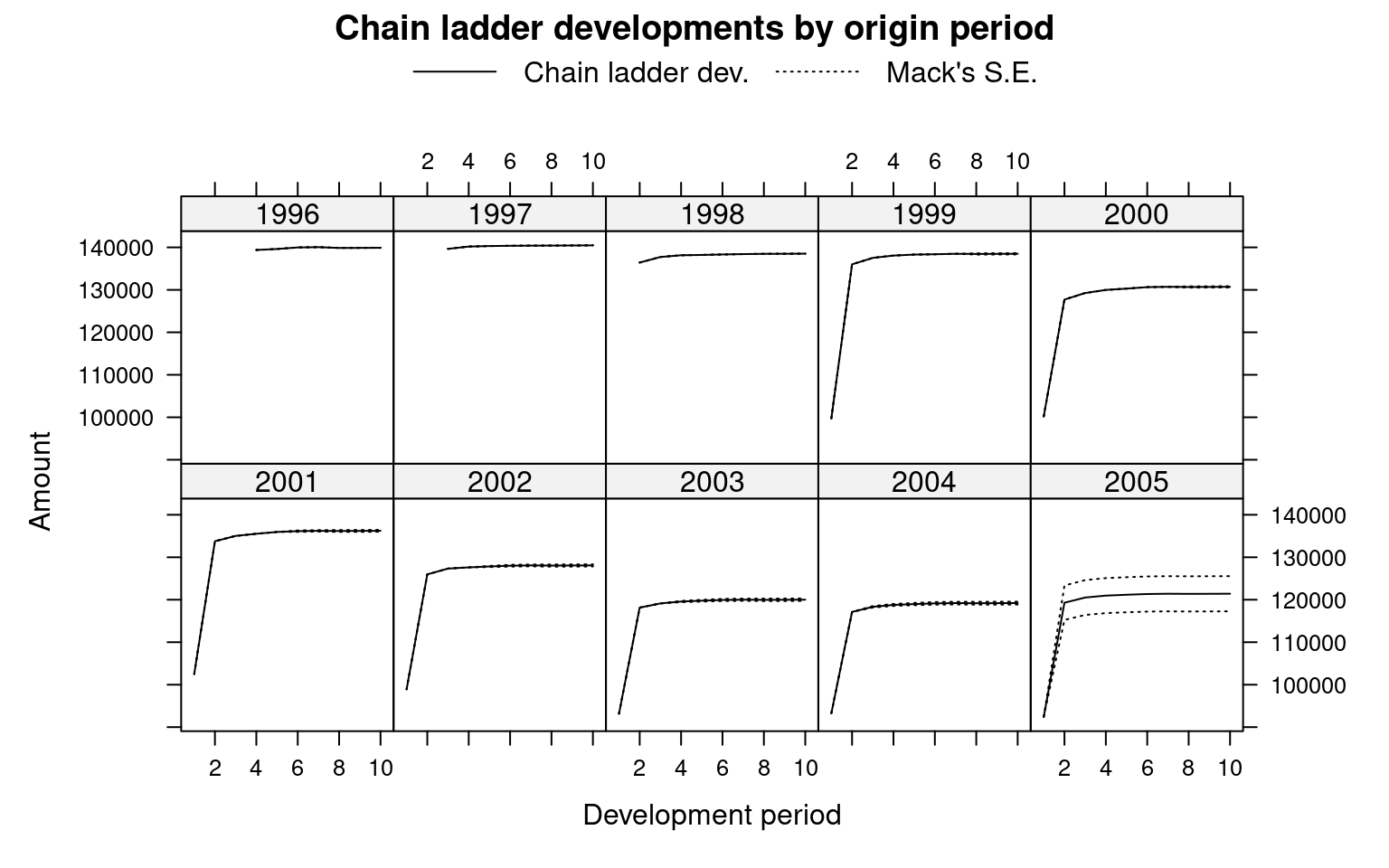
For more similar triangles datasets, see nortritpl8800 (import with data("ausprivauto0405")): Australian liabilty insurance triangles dataset, sgautoprop9701: Singapore general liability triangles dataset (import with data("norauto")), swtri1auto: Switzerland general liability triangles dataset (import with data("beMTPL16")), or usautotri9504 (import with data("pg17trainpol")): US Automobile triangles dataset.