Frequency analysis with a Zero Inflated Regression of a French Motor Third Party Liability dataset

Siharath Julien

2024-09-01

Introduction

Session Settings

# Graphs----
face_text='plain'
face_title='plain'
size_title = 14
size_text = 11
legend_size = 11

global_theme <- function() {
  theme_minimal() %+replace%
    theme(
      text = element_text(size = size_text, face = face_text),
      legend.position = "bottom",
      legend.direction = "horizontal", 
      legend.box = "vertical",
      legend.key = element_blank(),
      legend.text = element_text(size = legend_size),
      axis.text = element_text(size = size_text, face = face_text), 
      plot.title = element_text(
        size = size_title, 
        hjust = 0.5
      ),
      plot.subtitle = element_text(hjust = 0.5)
    )
}

# Outputs
options("digits" = 2)

In Brief

In some instances, zeros appear frequently in the data, indicating a specific structure that a simple Poisson model fails to account for, leading to biased and inaccurate estimates. To address this issue, we employ zero-inflated regression models, which are designed to handle datasets with an excess of zero counts by modeling both the occurrence of zeros and the count data separately.

The purpose of this vignette is to illustrate the application of zero-inflated regression in the analysis of insurance data, specifically using the freMTPL6 dataset from Charpentier (2014). This dataset comprises detailed information on insurance contracts and claims related to French motor third-party liability insurance. By applying zero-inflated regression, we aim to accurately model the frequency of claims and investigate the factors that influence claim occurrences within this insurance data, providing a more nuanced understanding than standard count models.

Required Packages

Show the code

required_libraries <- c(
  "tidyverse",
  "CASdatasets",
  "pscl",
  "splines",
  "AER",
  "broom",
  "knitr",
  "kableExtra"
)
invisible(lapply(required_libraries, library, character.only = TRUE))

Data

The data used in this vignette are sourced from a French motor third-party liability insurance portfolio.

The dataset, freMPL6, contains comprehensive details on insurance contracts and client information, obtained from a French insurance company. This dataset specifically pertains to a motor insurance portfolio, providing valuable insights into the characteristics and behavior of policyholders within this segment of the insurance market.

Dictionaries

The list of the 20 variables from the freMPL6 dataset is reported in Table 1.

Table 1: Content of the freMPL6 dataset

Attribute	Type	Description
Exposure	Numeric	The exposure, in years
LicAge	Numeric	The driving license age, in months
RecordBeg	Date	Beginning date of record
RecordEnd	Date	End date of record
Gender	Factor	Gender of the driver, either “Male” or “Female”
MariStat	Factor	Marital status of the driver, either “Alone” or “Other”
SocioCateg	Factor	Socio-economic category of the driver, known as CSP in France, between “CSP1” and “CSP99”
VehUsage	Factor	Usage of the vehicle, among “Private”, “Private+trip to office”, “Professional”, “Professional run”
DrivAge	Numeric	Age of the driver, in years
HasKmLimit	Boolean	Indicator if there’s a mileage limit for the policy, 1 if yes, 0 otherwise
ClaimAmount	Numeric	Total claim amount of the guarantee
ClaimNbResp	Numeric	Number of responsible claims in the 4 preceding years
ClaimNbNonResp	Numeric	Number of non-responsible claims in the 4 preceding years
ClaimNbParking	Numeric	Number of parking claims in the 4 preceding years
ClaimNbFireTheft	Numeric	Number of fire-theft claims in the 4 preceding years
ClaimNbWindscreen	Numeric	Number of windscreen claims in the 4 preceding years
OutUseNb	Numeric	Number of out-of-use instances in the 4 preceding years
RiskArea	Numeric	Unknown risk area, between 1 and 13, possibly ordered
BonusMalus	Numeric	Bonus-malus coefficient, between 50 and 350: <100 means bonus, >100 means malus in France
ClaimInd	Boolean	Claim indicator of the guarantee (this is not the claim number)

Importation

code for importing our datasets

data("freMPL6")

freMPL6$DrivAgefactor <- cut(freMPL6$DrivAge,
                        breaks = c(-Inf, 25, 40, 60, 70, Inf),
                        labels = c("18-25","25-40", "40-60", "50-70", "70+"),
                        right = FALSE)

Models

Purpose

In the context of insurance, Zero-inflated regression models, such as Zero-inflated Poisson (ZIP) and Zero-inflated Negative Binomial (ZINB), are essential tools for gaining a more nuanced understanding of data compared to simple Poisson regression. These models are particularly advantageous when dealing with datasets that exhibit an excess of zeros, as they differentiate between zeros that result from structural causes (e.g., policyholders who never file claims) and those that occur by random chance.

Zero-inflated models are especially useful when analyzing variables that influence the likelihood of filing a claim, such as a driver’s age, gender, or driving history. These factors often have varying propensities to result in zero claims, which may stem from inherent characteristics of specific driver profiles or particular usage patterns. By explicitly modeling both the zero-generating process and the claim-generating process, zero-inflated regression models provide more accurate estimates and predictions. This allows insurers to enhance risk assessments, refine pricing strategies, and make more informed decisions.

In fields like insurance claims analysis, healthcare data analytics, and ecological studies—where understanding the relationship between multiple variables and the occurrence of events (such as claims or incidents) is crucial—these models excel at capturing the complexities of the data. They enable a more precise analysis of how different factors influence the likelihood of events, leading to better-targeted products and pricing strategies. Ultimately, this improves the ability to manage risk and optimize profitability.

In this analysis, we will investigate the relationship between the response variable ClaimNbResp (which represents the number of claims where the driver is deemed responsible) and various explanatory variables, including DrivAge (driver’s age), Gender, LicAge (age of the driving license), BonusMalus (driver’s bonus-malus score), and VehUsage (vehicle usage type). This modeling approach is consistent with the principles advocated by Agresti (2013), a renowned authority in statistical methodology, who underscores the significance of incorporating multiple explanatory factors in regression analysis. By including these variables in our model, we aim to gain a deeper understanding of how these factors influence the likelihood of a driver being responsible for a claim.

Modeling Insurance Claim Frequency with Zero-Inflated Negative Binomial Regression

To model the frequency of insurance claims, we utilize a Zero-Inflated Negative Binomial (ZINB) Regression approach for the response variable ClaimNbResp, which represents the count of insurance claims and is typically assumed to follow a Poisson distribution:

$$\text{ClaimNbResp} \sim \text{Poisson}(\mu),$$

where $\mu$ represents the mean rate of claims. The ZINB approach is particularly well-suited for handling overdispersed data with excess zeros, offering a flexible, nonlinear modeling framework. Specifically, we express the natural logarithm of $\mu$ as a linear combination of predictor variables, along with an adjustment for exposure:

$$\log(\mu) = \beta_0 + \beta_1 \times \text{DrivAge} + \beta_2 \times \text{Gender} + \beta_3 \times \text{LicAge} +$$$$\beta_4 \times \text{BonusMalus} + \beta_5 \times \text{VehUsage} + \log(\text{Exposure}),$$

where DrivAge denotes the driver’s age, Gender is a binary variable indicating the driver’s gender, LicAge represents the age of the driving license, BonusMalus captures the driver’s bonus-malus score, VehUsage reflects the type of vehicle usage, and $\log(\text{Exposure})$ adjusts for the exposure variable. The coefficients $\beta_0, \beta_1, \beta_2, \beta_3, \beta_4, \beta_5$ are parameters to be estimated through the regression process.

In addition to the count component, the zero-inflation part of the model accounts for the probability of excess zeros via a logistic regression model:

$$\text{Logit}(P(\text{zero})) = Z\gamma,$$

where $Z$ represents the matrix of covariates for the zero-inflation model, and $\gamma$ is the vector of coefficients associated with these covariates.

In this framework, the intercept $\beta_0$ and the coefficients $\beta_1, \beta_2, \beta_3, \beta_4, \beta_5$ are estimated to quantify their effects on the expected rate of claims. The logistic regression component for zero inflation enhances the model’s capacity to capture complex, nonlinear relationships and the presence of excess zeros in the data, resulting in a more flexible and accurate model fit.

Pay Attention

The results from Zero-inflated regression models are valid under the following conditions:

• The responses are independent.
• The responses follow a Poisson distribution with parameter $\lambda$.
• There may be overdispersion present in the data.

The estimated $\mu$ parameter, which represents the mean of claims, is 0.27.

set.seed(1234) 

theoretic_count <- rpois(nrow(freMPL6), mean(freMPL6$ClaimNbResp))

tc_df <- tibble(theoretic_count)

freq_theoretic <- prop.table(table(tc_df$theoretic_count))

freq_claim <- prop.table(table(freMPL6$ClaimNbResp))

freq_theoretic_df <- tibble(
  Count = as.numeric(names(freq_theoretic)),
  Frequency = as.numeric(freq_theoretic),
  Source = "Theoretical Count"
)

freq_claim_df <- tibble(
  Count = as.numeric(names(freq_claim)),
  Frequency = as.numeric(freq_claim),
  Source = "Empirical Count"
)

freq_combined <- freq_theoretic_df |> 
  rbind(freq_claim_df)

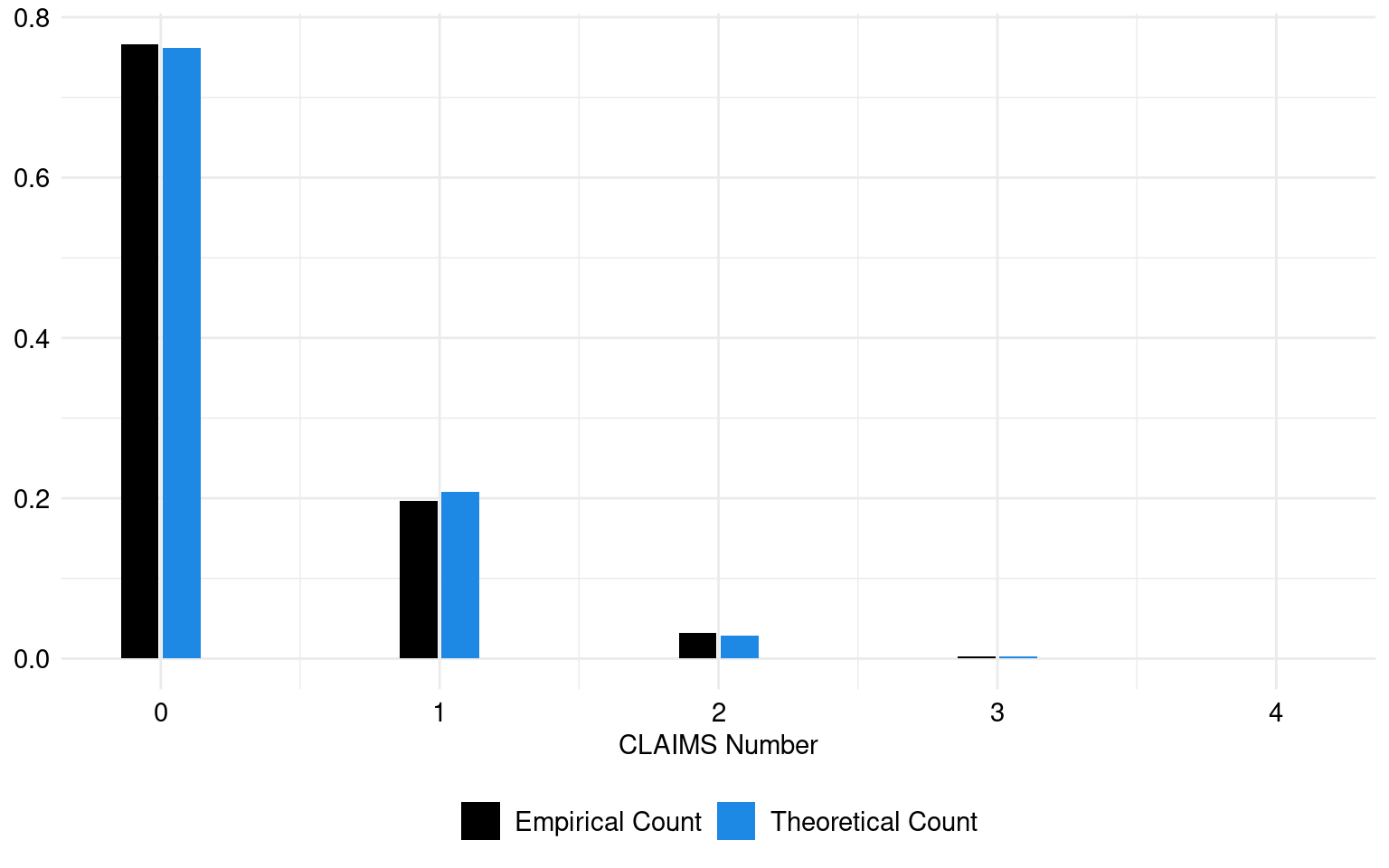
The theoretical and empirical histograms associated with a Poisson distribution are shown in Figure 1.

Code for the following graph

ggplot(freq_combined, aes(x = Count, y = Frequency, fill = Source)) +
  geom_bar(stat = "identity", position = "dodge2", width = 0.3) +
  labs(x = "CLAIMS Number", y = "Frequency", fill = "Legend") +
  theme(legend.position = "right") +
  scale_fill_manual(
    NULL,
    values = c("Empirical Count" = "black", "Theoretical Count" = "#1E88E5")
  ) +
  labs(fill = "Legend") +
  labs(x = "CLAIMS Number", y = NULL) +
  theme(legend.position = "right")+
  global_theme()

Figure 1: Theoretical and empirical histogram of claims in frequence

freg <- formula(ClaimNbResp ~ DrivAgefactor + LicAge
                + Gender + BonusMalus +  MariStat
                + VehUsage + offset(Exposure)|
                  Gender + DrivAgefactor + BonusMalus + LicAge)

reg <- zeroinfl(freg, data = freMPL6, dist = "poisson")

summary(reg)

Call:
zeroinfl(formula = freg, data = freMPL6, dist = "poisson")

Pearson residuals:
   Min     1Q Median     3Q    Max
-3.647 -0.469 -0.387 -0.199 43.154

Count model coefficients (poisson with log link):
                                Estimate Std. Error z value Pr(>|z|)
(Intercept)                    -3.963510   0.090390  -43.85  < 2e-16 ***
DrivAgefactor25-40             -0.586757   0.064947   -9.03  < 2e-16 ***
DrivAgefactor40-60             -0.263728   0.075345   -3.50  0.00046 ***
DrivAgefactor50-70             -0.253096   0.093989   -2.69  0.00708 **
DrivAgefactor70+               -0.217151   0.106506   -2.04  0.04146 *
LicAge                          0.001951   0.000145   13.47  < 2e-16 ***
GenderMale                     -0.068416   0.024663   -2.77  0.00554 **
BonusMalus                      0.029305   0.000507   57.78  < 2e-16 ***
MariStatOther                   0.180236   0.028675    6.29  3.3e-10 ***
VehUsagePrivate+trip to office  0.175531   0.029457    5.96  2.5e-09 ***
VehUsageProfessional            0.373158   0.032901   11.34  < 2e-16 ***
VehUsageProfessional run        0.562056   0.059676    9.42  < 2e-16 ***

Zero-inflation model coefficients (binomial with logit link):
                    Estimate Std. Error z value Pr(>|z|)
(Intercept)         3.28e+01   2.01e+00   16.26  < 2e-16 ***
GenderMale          1.46e-01   9.70e-02    1.51  0.13102
DrivAgefactor25-40 -1.43e+01   9.39e-01  -15.19  < 2e-16 ***
DrivAgefactor40-60 -1.58e+01   9.41e-01  -16.82  < 2e-16 ***
DrivAgefactor50-70 -1.60e+01   9.69e-01  -16.54  < 2e-16 ***
DrivAgefactor70+   -1.62e+01   9.90e-01  -16.37  < 2e-16 ***
BonusMalus         -3.68e-01   2.23e-02  -16.47  < 2e-16 ***
LicAge              2.17e-03   6.36e-04    3.41  0.00066 ***
---
Signif. codes:  0 '***' 0.001 '**' 0.01 '*' 0.05 '.' 0.1 ' ' 1

Number of iterations in BFGS optimization: 39
Log-likelihood: -2.52e+04 on 20 Df

This Zero-Inflated regression model is used to predict NbClaim (number of claims) with DrivAge,LicAge , Gender, MariStat (marital status), BonusMalus, and VehUsage as predictor variables.

Count Model (Poisson with Log Link):

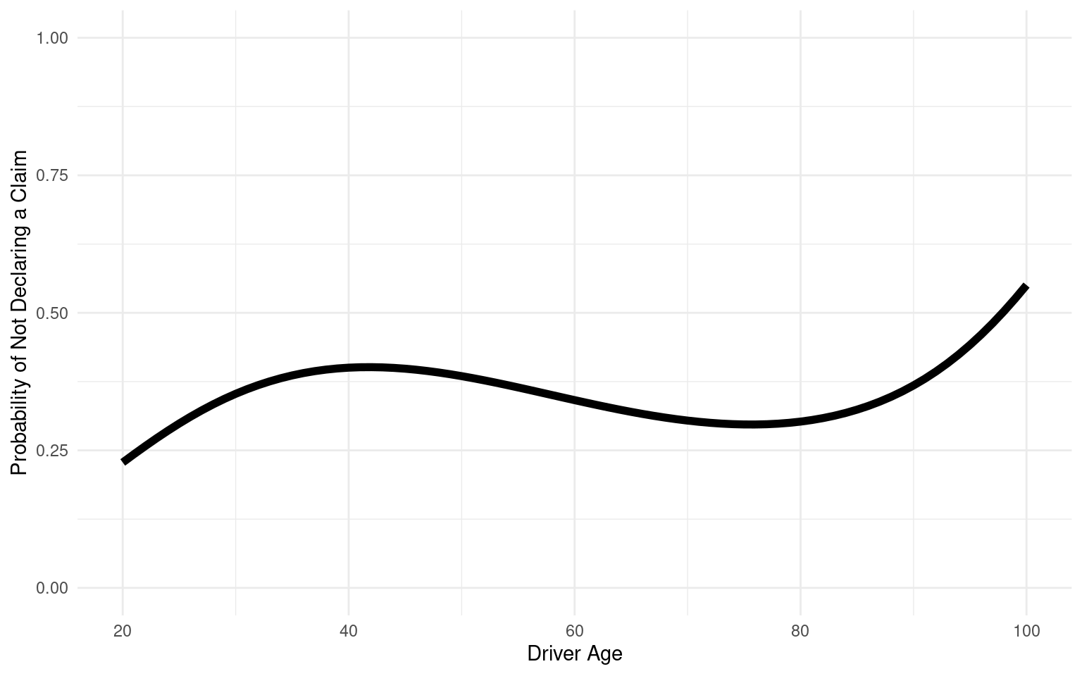
In the count component of the model, the coefficients represent the estimated change in the log count of responsible claims (ClaimNbResp) associated with each predictor level, relative to a reference level. For instance, the coefficients for drivers aged 25-40, 40-60, 50-70, and 70+ are all negative compared to the reference group (drivers younger than 25), indicating that older drivers are associated with a lower log count of responsible claims. The statistical significance of these coefficients (p < 0.05) underscores their importance in predicting the frequency of responsible claims, suggesting that age is a key factor in claim occurrence.

Zero-Inflation Model (Binomial with Logit Link):

The coefficients in the zero-inflation component model the log-odds of observing excess zeros (zero-inflation) versus non-excess zeros. The results indicate that older age groups (25-40, 40-60, 50-70, 70+) significantly reduce the log-odds of zero-inflation compared to the reference group (drivers younger than 25). This implies that younger drivers are more likely to contribute to the excess zeros in the data, potentially due to not filing claims despite having a higher risk profile.

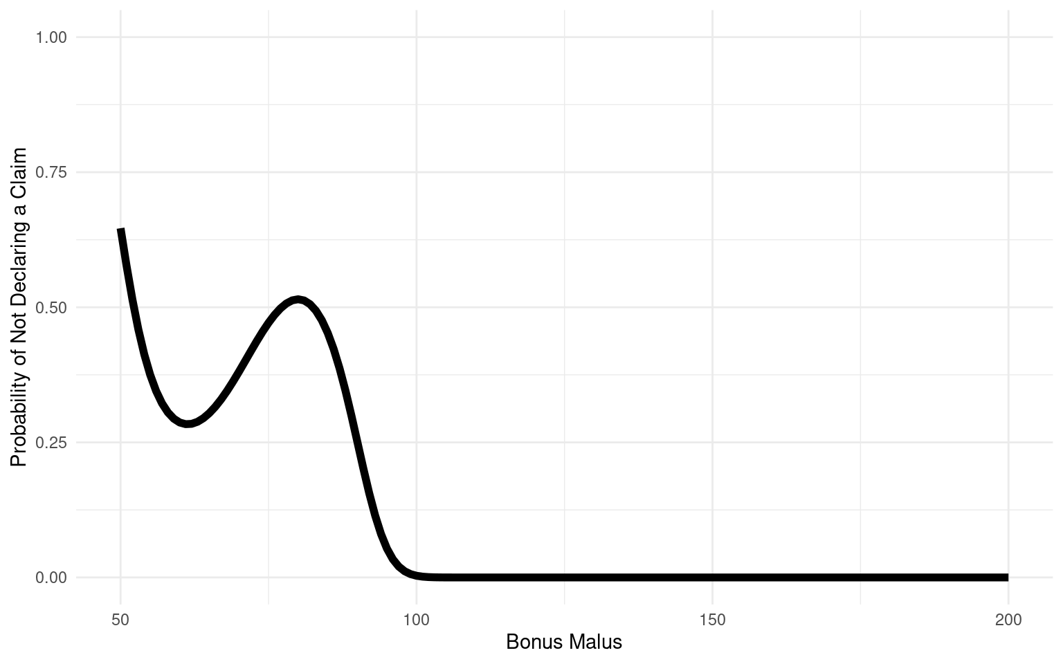
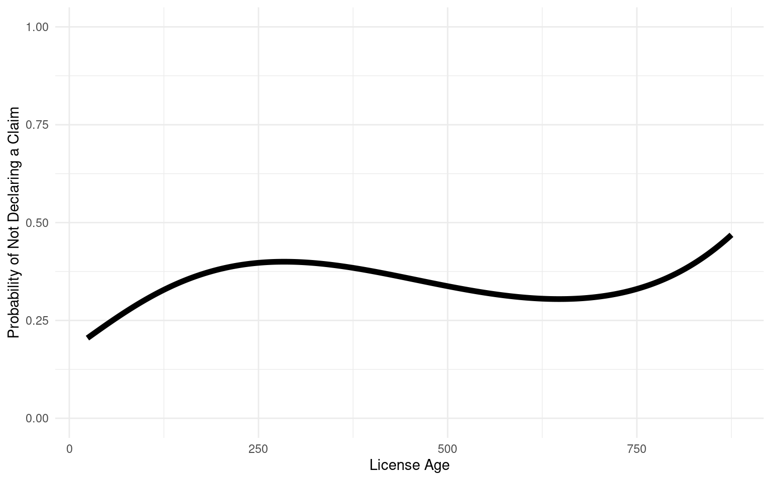
The variables LicAge and BonusMalus also influence zero-inflation, with LicAge slightly increasing the log-odds of zero-inflation, suggesting that more experienced drivers might be more likely to contribute to the excess zeros. Conversely, BonusMalus significantly decreases the log-odds, indicating that drivers with higher bonus-malus scores are less likely to contribute to the excess zeros. Interestingly, the Gender variable (Male) is not statistically significant in the zero-inflation model, suggesting that gender may not be a strong predictor of whether a claim is filed or not.

This analysis provides valuable insights into the factors that influence both the frequency of responsible claims and the likelihood of zero-inflation in the dataset, allowing for more nuanced risk assessments and pricing strategies.

• Count
• Zero

• • Coefficients
  • Count-Ratio and Confidence intervals

  Code to create the table

  summary_reg <- summary(reg)
  
  # Create a tidy data frame for the count model coefficients
  tidy_count <- summary_reg$coefficients$count |>
    as.data.frame() |>
    mutate(significance = case_when(
      `Pr(>|z|)` < 0.001 ~ "***",
      `Pr(>|z|)` < 0.01 ~ "**",
      `Pr(>|z|)` < 0.05 ~ "*",
      `Pr(>|z|)` < 0.1 ~ ".",
      TRUE ~ ""
    ))
  
  kable(tidy_count, format = "html", escape = FALSE) |>
    kable_styling(full_width = FALSE) |>
    add_footnote(c("Significance levels : *** p < 0.001, ** p < 0.01, * p < 0.05, . p < 0.1"),
                 notation = "none")

  Table 2: Coefficients for the Count model

  	Estimate	Std. Error	z value	Pr(>|z|)	significance
  (Intercept)	-3.96	0.09	-43.9	0.00	***
  DrivAgefactor25-40	-0.59	0.06	-9.0	0.00	***
  DrivAgefactor40-60	-0.26	0.08	-3.5	0.00	***
  DrivAgefactor50-70	-0.25	0.09	-2.7	0.01	**
  DrivAgefactor70+	-0.22	0.11	-2.0	0.04	*
  LicAge	0.00	0.00	13.5	0.00	***
  GenderMale	-0.07	0.02	-2.8	0.01	**
  BonusMalus	0.03	0.00	57.8	0.00	***
  MariStatOther	0.18	0.03	6.3	0.00	***
  VehUsagePrivate+trip to office	0.18	0.03	6.0	0.00	***
  VehUsageProfessional	0.37	0.03	11.3	0.00	***
  VehUsageProfessional run	0.56	0.06	9.4	0.00	***
  Significance levels : *** p < 0.001, ** p < 0.01, * p < 0.05, . p < 0.1

  Code to create the table

  estimates <- summary_reg$coefficients$count[-1, ] 
  
  exp_estimates <- exp(estimates[, "Estimate"])
  
  p_values <- estimates[, "Pr(>|z|)"]
  
  conf_int <- confint(reg)
  
  conf_int_exp <- exp(conf_int)
  
  reg_count_ratio <- data.frame(
    count_ratio = round(exp_estimates, 2),
    `CI 2.5` = conf_int_exp[2:12, 1],
    `CI 97.5` = conf_int_exp[2:12, 2],
    p.value = p_values
  )
  
  reg_count_ratio <- reg_count_ratio |>
    mutate(significance = case_when(
      p.value < 0.001 ~ "***",
      p.value < 0.01 ~ "**",
      p.value < 0.05 ~ "*",
      p.value < 0.1 ~ ".",
      TRUE ~ ""
    )) |>
    dplyr::select(-p.value)
  
  kable(reg_count_ratio, format = "html", escape = FALSE, digits = 2) |>
    kable_styling(full_width = FALSE) |>
    add_footnote(c("Significance levels: *** p < 0.001, ** p < 0.01, * p < 0.05, . p < 0.1"),
                 notation = "none")

  Table 3: Count Ratio and confidence intervals for the Count model

  	count_ratio	CI.2.5	CI.97.5	significance
  DrivAgefactor25-40	0.56	0.49	0.63	***
  DrivAgefactor40-60	0.77	0.66	0.89	***
  DrivAgefactor50-70	0.78	0.65	0.93	**
  DrivAgefactor70+	0.80	0.65	0.99	*
  LicAge	1.00	1.00	1.00	***
  GenderMale	0.93	0.89	0.98	**
  BonusMalus	1.03	1.03	1.03	***
  MariStatOther	1.20	1.13	1.27	***
  VehUsagePrivate+trip to office	1.19	1.13	1.26	***
  VehUsageProfessional	1.45	1.36	1.55	***
  VehUsageProfessional run	1.75	1.56	1.97	***
  Significance levels: *** p < 0.001, ** p < 0.01, * p < 0.05, . p < 0.1

  Each count ratio reflects the change in the odds of making a responsible claim (ClaimNbResp) associated with a one-unit increase in the predictor variable, relative to the reference category. For example, a count ratio of 0.56 for drivers aged 25-40 indicates that the odds of making a responsible claim for this age group are approximately -44% lower compared to the reference category, which consists of drivers younger than 25. Similarly, for drivers aged 40-60, the odds decrease by -23% relative to the reference category.

  However, as drivers age beyond 60, the data suggests that the likelihood of making a responsible claim increases. This pattern indicates that while middle-aged drivers (25-60) have lower odds of making a responsible claim compared to younger drivers, the odds begin to rise in older age groups, suggesting an increased risk of responsible claims as age advances.

• Coefficents
• Count-Ratio and Confidence intervals

code to create the table

# Create a tidy data frame for the zero-inflation model coefficients
tidy_zero <- summary_reg$coefficients$zero |>
  as.data.frame() |>
  mutate(significance = case_when(
    `Pr(>|z|)` < 0.001 ~ "***",
    `Pr(>|z|)` < 0.01 ~ "**",
    `Pr(>|z|)` < 0.05 ~ "*",
    `Pr(>|z|)` < 0.1 ~ ".",
    TRUE ~ ""
  ))

kable(tidy_zero, format = "html", escape = FALSE) |>
  kable_styling(full_width = FALSE) |>
  add_footnote(c("Significance levels : *** p < 0.001, ** p < 0.01, * p < 0.05, . < 0.05"),
               notation = "none")

Table 4: Coefficients for the Zero model

	Estimate	Std. Error	z value	Pr(>|z|)	significance
(Intercept)	32.76	2.01	16.3	0.00	***
GenderMale	0.15	0.10	1.5	0.13
DrivAgefactor25-40	-14.27	0.94	-15.2	0.00	***
DrivAgefactor40-60	-15.83	0.94	-16.8	0.00	***
DrivAgefactor50-70	-16.03	0.97	-16.5	0.00	***
DrivAgefactor70+	-16.21	0.99	-16.4	0.00	***
BonusMalus	-0.37	0.02	-16.5	0.00	***
LicAge	0.00	0.00	3.4	0.00	***
Significance levels : *** p < 0.001, ** p < 0.01, * p < 0.05, . < 0.05

Code to create the table

estimates <- summary_reg$coefficients$zero[-1, ]

exp_estimates <- exp(estimates[, "Estimate"])

p_values <- estimates[, "Pr(>|z|)"]

conf_int <- confint(reg)

conf_int_exp <- exp(conf_int)

reg_count_ratio <- data.frame(
  count_ratio = exp_estimates,
  `CI 2.5` = conf_int_exp[13:19, 1],
  `CI 97.5` = conf_int_exp[13:19, 2],
  p.value = p_values
)

reg_count_ratio <- reg_count_ratio |>
  mutate(significance = case_when(
    p.value < 0.001 ~ "***",
    p.value < 0.01 ~ "**",
    p.value < 0.05 ~ "*",
    p.value < 0.1 ~ ".",
    TRUE ~ ""
  )) |>
  dplyr::select(-p.value)

kable(reg_count_ratio, format = "html", escape = FALSE) |>
  kable_styling(full_width = FALSE) |>
  add_footnote(c("Significance levels: *** p < 0.001, ** p < 0.01, * p < 0.05, . p < 0.1"),
               notation = "none")

Table 5: Count-Ratio and Confidence intervals for the Zero model

	count_ratio	CI.2.5	CI.97.5	significance
GenderMale	1.16	3.3e+12	8.8e+15
DrivAgefactor25-40	0.00	9.6e-01	1.4e+00	***
DrivAgefactor40-60	0.00	0.0e+00	0.0e+00	***
DrivAgefactor50-70	0.00	0.0e+00	0.0e+00	***
DrivAgefactor70+	0.00	0.0e+00	0.0e+00	***
BonusMalus	0.69	0.0e+00	0.0e+00	***
LicAge	1.00	6.6e-01	7.2e-01	***
Significance levels: *** p < 0.001, ** p < 0.01, * p < 0.05, . p < 0.1

Graphs

• Count Model
• Zero Model

• Code to create the following graph

  estimates <- summary_reg$coefficients$count[-1, ] 
  
  count_ratio <- exp(estimates[, "Estimate"])
  
  conf_int <- exp(confint(reg))[-1, ]
  
  vars_count <- grep("^(DrivAge|Gender|LicAge|MariStat|VehUsage)", names(count_ratio), value = TRUE)
  
  vars_count_with_count <- paste0("count_", vars_count)
  
  data_age <- tibble(
    variable = vars_count,
    coefficient = count_ratio[vars_count], 
    lower_bound = conf_int[vars_count_with_count, 1], 
    upper_bound = conf_int[vars_count_with_count, 2]
  )
  
  data_age$variable <- factor(data_age$variable, levels = rev(vars_count))
  
  
  ggplot(
    data_age, 
    aes(
      x = coefficient,
      y = variable,
      xmin = lower_bound,
      xmax = upper_bound
    )
  ) +
    geom_point(stat = "identity", size = 3, color = "#1E88E5") +
    geom_errorbar(
      width = 0.2,
      position = position_dodge(width = 0.6),
      color = "#1E88E5"
    ) +
    geom_vline(xintercept = 1, color = "black", linetype = "solid") +
    labs(
      x = NULL,
      y = NULL
    ) +
    global_theme()

  Figure 2: Counts ratio and confidence intervals of the count model

  

We will utilize splines to visualize the impact of BonusMalus, LicAge, and DrivAge on the non-claiming rate. Splines, which are piecewise polynomial functions, provide a powerful tool for smoothing and capturing non-linear relationships that linear models may fail to detect.

In the context of claim regression, splines are particularly effective for modeling the complex, non-linear effects of factors such as age, income, or policy duration on the likelihood or frequency of claims. By allowing the model to adapt flexibly to the data’s underlying structure, this approach enhances both the accuracy and fit of the model. Consequently, insurers can achieve more precise risk assessments and make more informed decisions regarding pricing and policy underwriting.

• Bonus Malus impact
• License Age Impact
• Age Impact

Code to create the following graph

regZIbm <- zeroinfl(ClaimNbResp ~ 1 | bs(BonusMalus), 
                    offset = log(Exposure), 
                    data = freMPL6, 
                    dist = "poisson", 
                    link = "logit")

Warning: glm.fit: fitted probabilities numerically 0 or 1 occurred

Code to create the following graph

C <- tibble(BonusMalus = 50:200, Exposure = 1)

pred0 <- regZIbm |> 
  predict(newdata = C, type = "zero")

Warning in bs(BonusMalus, degree = 3L, knots = numeric(0), Boundary.knots =
c(50L, : some 'x' values beyond boundary knots may cause ill-conditioned bases

Code to create the following graph

C |> 
  mutate(Prediction = pred0) |> 
  ggplot(aes(x = BonusMalus, y = Prediction)) +
  geom_line(size = 2) +
  labs(x = "Bonus Malus", y = "Probability of Not Declaring a Claim") +
  ylim(0, 1) +
  theme_minimal()

Warning: Using `size` aesthetic for lines was deprecated in ggplot2 3.4.0.
ℹ Please use `linewidth` instead.

Figure 3: Bonus Malus impact on Claim Non-Declaration

The plot reveals that when the Bonus-Malus score is below 100, indicating a bonus, there is a higher probability of not declaring a claim. As the Bonus-Malus score increases beyond 100, this probability declines sharply, suggesting that drivers with higher scores are more inclined to report a claim.

This trend may imply that drivers who have accumulated bonuses are more likely to avoid declaring claims in an effort to preserve their favorable score, thus minimizing the potential increase in their insurance premiums.

Code to create the following graph

regZIbm <- zeroinfl(ClaimNbResp ~ 1 | bs(LicAge), 
                    offset = log(Exposure), 
                    data = freMPL6, 
                    dist = "poisson", 
                    link = "logit")

A <- tibble(LicAge = min(freMPL6$LicAge):max(freMPL6$LicAge), Exposure = 1)

pred0 <- regZIbm |> 
  predict(newdata = A, type = "zero")

A |> 
  mutate(Prediction = pred0) |>
  ggplot(aes(x = LicAge, y = Prediction)) +
  geom_line(size = 2) +
  labs(x = "License Age", y = "Probability of Not Declaring a Claim") +
  ylim(0, 1) +
  theme_minimal()

Figure 4: License Age impact on Claim Non-Declaration

Code to create the following graph

regZIbm <- zeroinfl(ClaimNbResp ~ 1 | bs(DrivAge), 
                    offset = log(Exposure), 
                    data = freMPL6, 
                    dist = "poisson", 
                    link = "logit")

B <- tibble(DrivAge = 20:100, Exposure = 1)

pred0 <- predict(regZIbm, newdata = B, type = "zero")

Warning in bs(DrivAge, degree = 3L, knots = numeric(0), Boundary.knots = c(20L,
: some 'x' values beyond boundary knots may cause ill-conditioned bases

Code to create the following graph

B |>
  mutate(Prediction = pred0) |>
  ggplot(aes(x = DrivAge, y = Prediction)) +
  geom_line(size = 2) +
  labs(x = "Driver Age", y = "Probability of Not Declaring a Claim") +
  ylim(0, 1) +
  theme_minimal()

Figure 5: Age impact on Claim Non-Declaration

References

Agresti, Alan. 2013. Categorical Data Analysis, 3rd Edition.

Charpentier, Arthur. 2014. Computational Actuarial Science with R. The R Series. Chapman; Hall/CRC. https://www.routledge.com/Computational-Actuarial-Science-with-R/Charpentier/p/book/9781138033788.

See also

For more similar claim frequency datasets with a Poisson-like distribution, see freMTPL (import with data("freMTPLfreq")): French automobile dataset, beMTPL16: Belgian automobile dataset (import with data("beMTPL16")), ausprivauto0405 (import with data("ausprivauto0405")): Australian automobile dataset, or pg17trainpol (import with data("pg17trainpol")).