Canadian life insurance

This dataset contains information of 14,889 contracts in force with a large Canadian insurer over the period December 29, 1988 through December 31, 1993. These contracts are joint and last-survivor annuities that were in the payout status over the observation period. For each contract, we have the date of birth, date of death (if applicable) and sex of each annuitant. Binary dummies for uncensored observations and exit times are also available.

Usage

data(canlifins)
data(canlifins2)

Format

canlifins is a data frame of 10 columns and 14,889 rows:

EntryAgeM

Entry age of the male.

DeathTimeM

Time of death of the male (zero if not applicable).

AnnuityExpiredM

The date that the annuity guarantee expired (if applicable).

IsDeadM

A binary indicating uncensored observation.

ExitAgeM

Exit age of the male.

EntryAgeF

Entry age of the female.

DeathTimeF

Time of death of the female (zero if not applicable).

AnnuityExpiredF

The date that the annuity guarantee expired (if applicable).

IsDeadF

A binary indicating uncensored observation.

ExitAgeF

Exit age of the female.

Originally in Frees et al. (1995), the dataset contains 22 contracts where both annuitants are male, 36 contracts where both annuitants are female, in addition to 14,889 contracts where one annuitant is male and the other female (so a total of 14,947 contracts).

canlifins2 is a data frame of 2 columns and 14,889 rows with either the observed death age in canlifins or simulated death age based on the residual survival time. Dependency between male and female is taken into account.

DeathAgeM

Death age of the male.

DeathAgeF

Death age of the female.

Source

Unknown private insurer.

References

Dataset used in Frees, Carriere and Valdez (1995), Annuity valuation with dependent mortality, Actuarial Research Clearing House 1995, Vol. 2, doi:10.2307/253744 .

Examples

# (1) load of data
#
data(canlifins)
dim(canlifins)
#> [1] 14889    10

# (2) Table 1 of Frees et al. (1995)
#

table(Age=cut(canlifins$EntryAgeM, c(0, 60, 70, 80, 120)), 
Status=cut(canlifins$DeathTimeM, c(-1, 0, 10)))
#>           Status
#> Age        (-1,0] (0,10]
#>   (0,60]     1166     42
#>   (60,70]    7598    534
#>   (70,80]    4347    806
#>   (80,120]    224    172
table(Age=cut(canlifins$EntryAgeF, c(0, 60, 70, 80, 120)), 
Status=cut(canlifins$DeathTimeF, c(-1, 0, 10)))
#>           Status
#> Age        (-1,0] (0,10]
#>   (0,60]     2940     30
#>   (60,70]    8190    238
#>   (70,80]    3004    242
#>   (80,120]    183     62


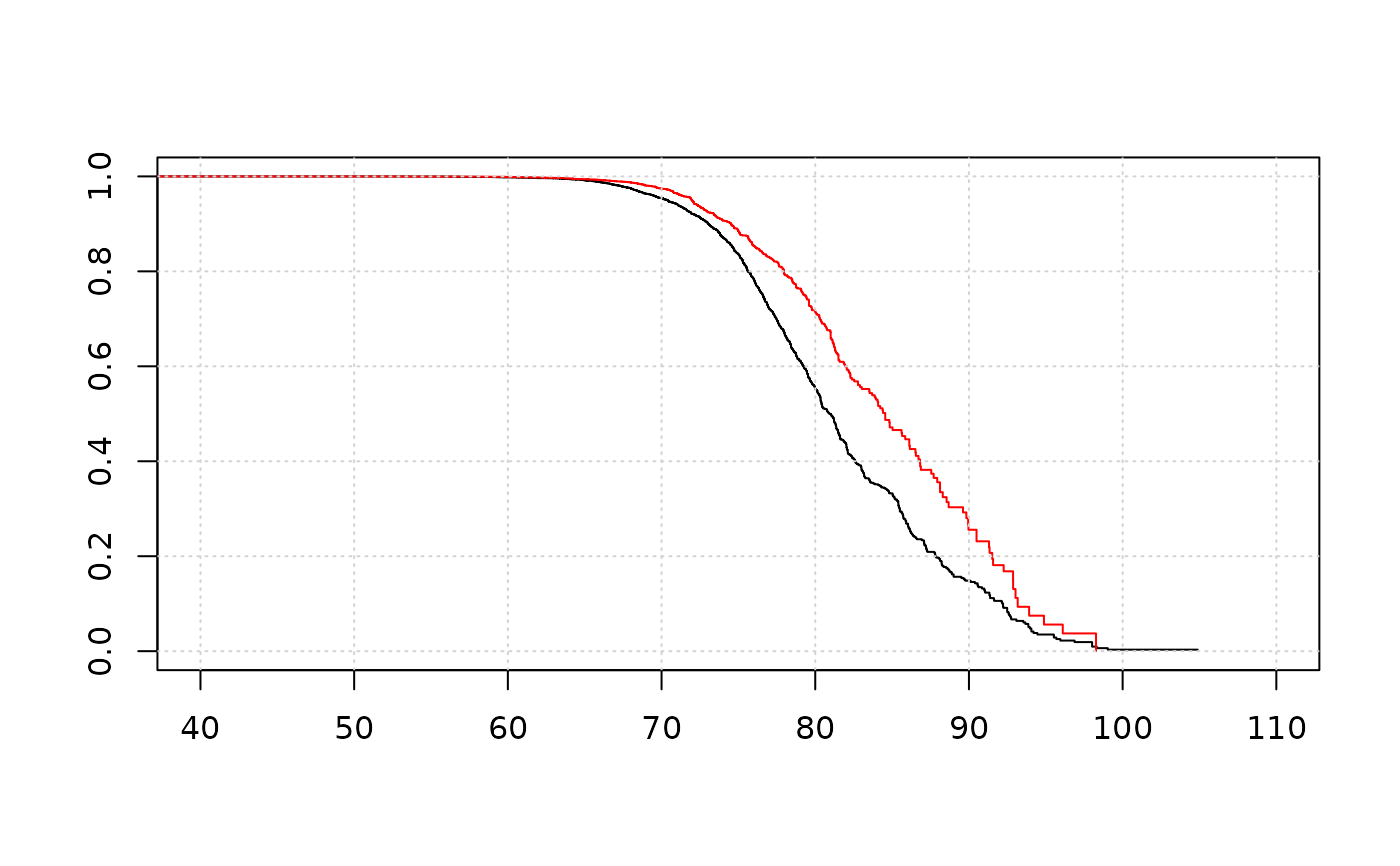
# (3) Figure 1 of Frees et al. (1995)
#

KMmale <- survfit(Surv(ExitAgeM, IsDeadM)~1, data=canlifins)
KMfemale <- survfit(Surv(ExitAgeF, IsDeadF)~1, data=canlifins)

plot(KMmale, xlim=c(40, 110), conf.int=FALSE)
lines(KMfemale, col="red", conf.int=FALSE)
grid()