Frequency analysis of a Belgian Motor Third Party Liability dataset

Siharath Julien

September, 2024

Introduction

Session Settings

# Graphs----
face_text='plain'
face_title='plain'
size_title = 14
size_text = 11
legend_size = 11

global_theme <- function() {
  theme_minimal() %+replace%
    theme(
      text = element_text(size = size_text, face = face_text),
      legend.position = "bottom",
      legend.direction = "horizontal", 
      legend.box = "vertical",
      legend.key = element_blank(),
      legend.text = element_text(size = legend_size),
      axis.text = element_text(size = size_text, face = face_text), 
      plot.title = element_text(
        size = size_title, 
        hjust = 0.5
      ),
      plot.subtitle = element_text(hjust = 0.5)
    )
}

# Outputs
options("digits" = 2)

In Brief

The objective of this vignette is to illustrate the practical application of Generalized Additive Models (GAM) in analyzing insurance data, with an emphasis on the beMTPL dataset from Charpentier (2014). Our focus lies in public liability for drivers, particularly in providing comprehensive insights into insurance contracts and claims associated with Belgium motor third-party liability insurance. Our objective is to develop a model to explore the factors that impact claim occurrences within the insurance dataset, with a special focus on the elderly.

Required Packages

Show the code

required_libraries <- c(
  "tidyverse", 
  "CASdatasets",
  "wesanderson",
  "mgcv",
  "broom",
  "knitr"
)
invisible(lapply(required_libraries, library, character.only = TRUE))

Data

The data used in this vignette come from the Belgium motor third-party liability insurance portfolio.

The dataset, beMTPL, encompasses details regarding contracts and clients obtained from a Belgium insurance company, related to a public liability insurance portfolio.

For convenience, the beMTPL table will be referred to as CLAIMS.

Dictionaries

The list of the 22 variables from the beMTPL dataset is reported in Table 1.

Table 1: Content of the beMTPL dataset: CLAIMS

Attribute	Type	Description
insurance_contract	Numeric	Unique identifier for the contract
policy_year	Numeric	Year of study or observation for the insured person
insured_year_birth	Numeric	insured’s year of birth
exposure	Numeric	Exposure duration in years
vehicle_age	Numeric	Age of the vehicle in years
policy_holder_age	Numeric	Seniority of the insured at the insurance agency
driver_license_age	Numeric	Age of the driver’s licence
vehicle_brand	Character	Brand of the vehicle
mileage	Numeric	Mileage of the vehicle
vehicle_power	Numeric	Power value of the vehicle
catalog_value	Numeric	Catalog value of the vehicle
claim_value	Numeric	Value of the claim
number_of_liability_claims	Numeric	Number of liability claims
number_of_bodily_injury_liability_claims	Numeric	Number of bodily injury liability claims
claim_time	Numeric	Time of the accident
claim_responsibility_rate	Numeric	Rate of responsibility for the claim (100% full responsibility, 0% no responsibility
driving_training_label	Bolean	Bolean indicating driving training
signal	Bolean	1 = warning, 0 = no warning

Importation

Code for importing our datasets

data(beMTPL16)

CLAIMS <- beMTPL16

CLAIMS <- CLAIMS |>
  mutate(insured_age = 2016 - insured_birth_year)

CLAIMS <- CLAIMS |>
  group_by(insurance_contract, policy_year) |>
  mutate(ClaimNB = sum(number_of_liability_claims == 1))

Models

Purpose

In the domain of public liability for automobile accidents, particularly with a focus on elderly drivers, Generalized Additive Models (GAM) are a reliable tool for understanding and predicting accident frequencies, repair costs, and claim patterns.

By employing GAM, insurers can better anticipate future challenges, refine pricing strategies, and enhance their resilience in an ever-evolving risk environment, specifically addressing the unique risks associated with elderly drivers.

In this analysis, we explore the relationship between the response variable target and the explanatory variables DriverAge and vehicle_age. This modeling framework aligns with the principles outlined by Agresti (2013), a prominent figure in statistical methodology, who emphasizes the importance of considering multiple explanatory factors in regression analysis.

To model the frequency of insurance claims, we employ a Generalized Additive Model (GAM) approach for the response variable ClaimNB, which represents the count of insurance claims and is assumed to follow a Quasi-Poisson distribution:

$$\text{ClaimNB} \sim \text{QuasiPoisson}(\lambda),$$

where $\lambda$ is the mean rate of claims. The GAM approach allows for flexible, nonlinear relationships between $\lambda$ and the predictor variables through the use of smooth functions. Specifically, we express the natural logarithm of $\lambda$ as a combination of these smooth functions and an additional term accounting for exposure:

$$\begin{equation} \log(\lambda_i) = \beta_0 + f_1(\text{insured age}_i) + f_2(\text{vehicle age}_i) + \log(\text{exposure}), \end{equation}$$

where $f_1(\text{insured age}_i)$, $f_2(\text{vehicle age}_i)$ are smooth functions of the predictor variables.

In this model, DriverAge represents the age of the insured individual, vehicle_age denotes the age of the vehicle, and $\log(\text{exposure})$ adjusts for the exposure variable. The intercept $\beta_0$ and the smooth functions $f_1$ and $f_2$ are estimated through regression to quantify their impact on the expected rate of claims. The smooth functions allow the model to capture complex, nonlinear relationships between the predictors and the response variable, providing a more flexible and accurate fit to the data.

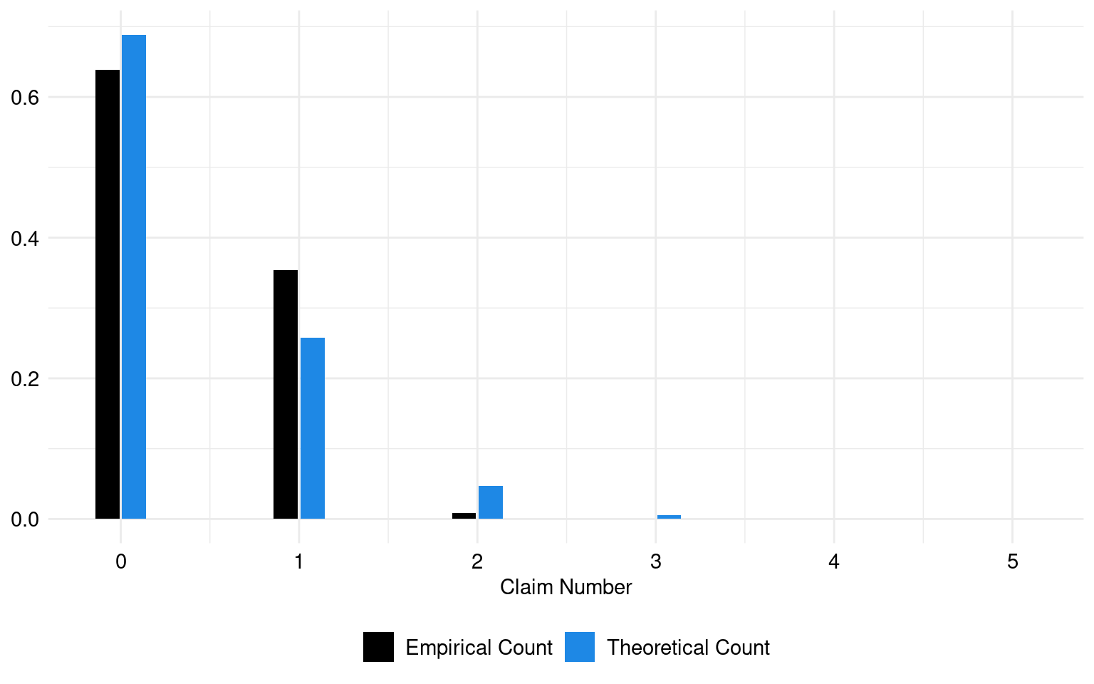
The estimated lambda parameter, which represents the mean of claims, is 0.37.

set.seed(1234) 

theoretic_count <- rpois(nrow(CLAIMS), mean(CLAIMS$ClaimNB))

tc_df <- tibble(theoretic_count)

freq_theoretic <- prop.table(table(tc_df$theoretic_count))

freq_claim <- prop.table(table(CLAIMS$ClaimNB))

freq_theoretic_df <- tibble(
  Count = as.numeric(names(freq_theoretic)),
  Frequency = as.numeric(freq_theoretic),
  Source = "Theoretical Count"
)

freq_claim_df <- tibble(
  Count = as.numeric(names(freq_claim)),
  Frequency = as.numeric(freq_claim),
  Source = "Empirical Count"
)

freq_combined <- freq_theoretic_df |> 
  rbind(freq_claim_df)

The theoretical and empirical histograms associated with a Poisson distribution are shown in Figure 1.

Code for the following graph

ggplot(freq_combined, aes(x = Count, y = Frequency, fill = Source)) +
  geom_bar(stat = "identity", position = "dodge2", width = 0.3) +
  labs(x = "Claim Number", y = "Frequency", fill = "Legend") +
  theme(legend.position = "right") +
  scale_fill_manual(
    NULL,
    values = c("Empirical Count" = "black", "Theoretical Count" = "#1E88E5")
  ) +
  labs(fill = "Legend") +
  labs(x = "Claim Number", y = NULL) +
  theme(legend.position = "right")+
  global_theme()

Figure 1: Theoretical and empirical histogram of claims in frequence

reg <- gam(
  ClaimNB ~ -1 + s(insured_age) + s(vehicle_age) + offset(log(exposure)),
  family = quasipoisson,
  data = CLAIMS
)

summary(reg)

Family: quasipoisson
Link function: log

Formula:
ClaimNB ~ -1 + s(insured_age) + s(vehicle_age) + offset(log(exposure))

Approximate significance of smooth terms:
                edf Ref.df   F p-value
s(insured_age) 4.80   5.78 105  <2e-16 ***
s(vehicle_age) 3.94   4.71 468  <2e-16 ***
---
Signif. codes:  0 '***' 0.001 '**' 0.01 '*' 0.05 '.' 0.1 ' ' 1

R-sq.(adj) =  -0.0915   Deviance explained =   -5%
GCV = 0.79694  Scale est. = 0.75161   n = 70791

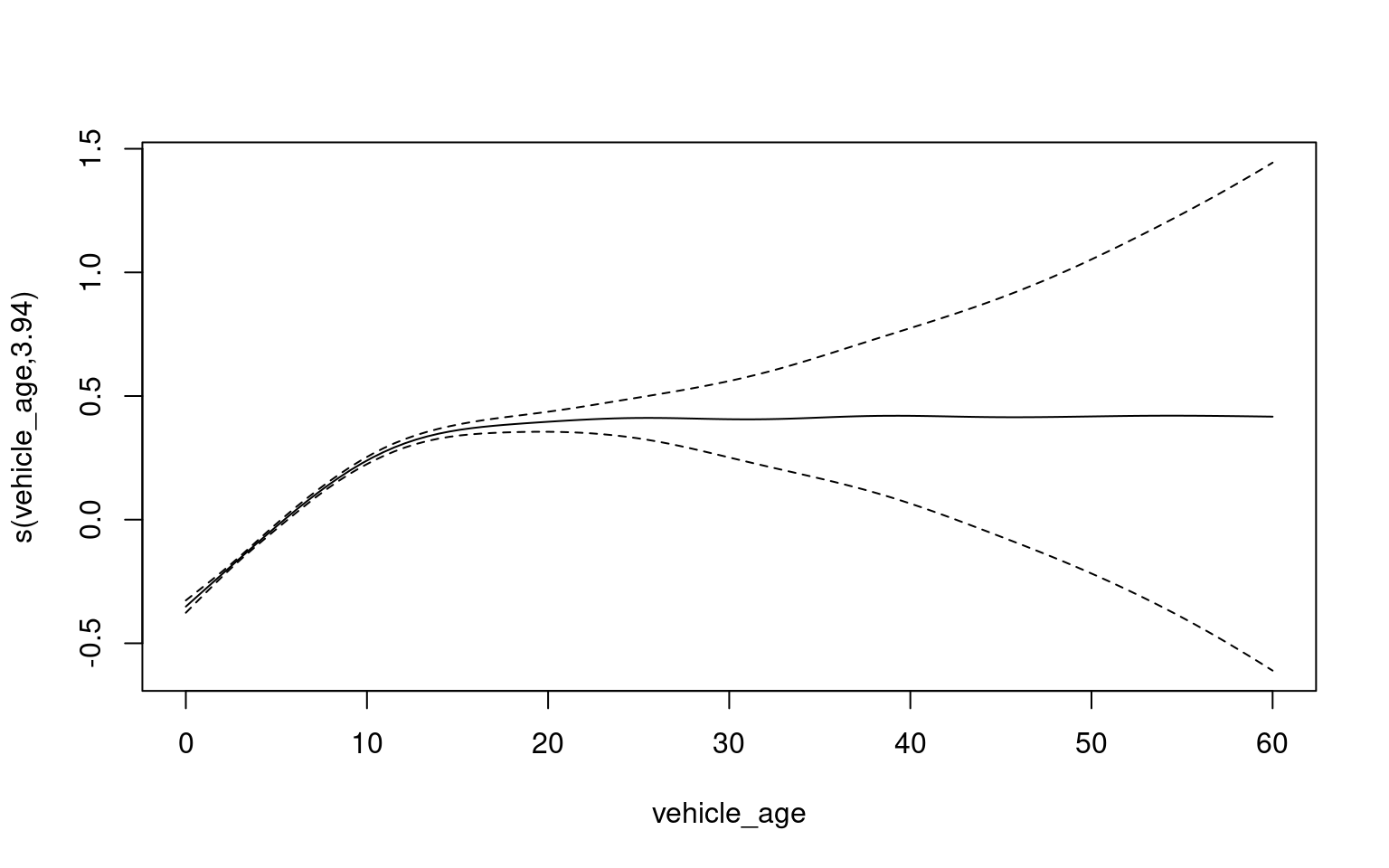
This generalized additive model (GAM) predicts the number of claims based on insured_age and vehicle_age as predictors. The smooth terms in the model are statistically significant, indicating that both insured_age and vehicle_age have a meaningful effect on the number of claims.

A positive coefficient for s(insured_age) suggests that increasing the age of the insured is associated with a higher expected log count of total liability claims. Similarly, the positive coefficient for s(vehicle_age) indicates that an increase in vehicle age is linked to a higher expected log count of claims.

Graphs

• DriverAge vehicle_age 3D perspective influence

• Code to create the following graph

  constant_offset <- mean(log(CLAIMS$exposure))
  
  
  pgam <- function(x1, x2){
    predict(
      reg,
      newdata = data.frame(
        vehicle_age = x1, 
        insured_age = x2, 
        exposure = exp(constant_offset)
      ),
      type = "response"
    )
  }
  
  M <- 31
  cx1 <- seq(from = min(CLAIMS$vehicle_age), to = max(CLAIMS$vehicle_age), length = M)
  cx2 <- seq(from = min(CLAIMS$insured_age), to = max(CLAIMS$insured_age), length = M)
  
  
  Pgam <- outer(cx1, cx2, Vectorize(pgam))
  
  
  persp(
    cx1, cx2, Pgam, theta = 30, phi = 20,
    xlab = "Vehicle Age", ylab = "Insured Age", zlab = "Predicted Claims",
    main = paste(
      "Predicted Claims with Constant Offset (log(exposure) =", 
      round(constant_offset, 2), ")"
    )
  )

  Figure 2: 3D impact perspective: DriverAge and vehicle_age

  

• DriverAge
• vehicle_age

• Code to create the following graph

  plot(reg, select = 1)

  Figure 3: Estimated effects of DriverAge

  

  The plot displays the smooth function of insured_age from the Generalized Additive Model (GAM). The solid line represents the estimated effect of insured_age on the log count of claims, with the dashed lines indicating 95% confidence intervals.

  • Trend: The effect of insured_age is relatively flat for ages 60 to 70, suggesting minimal impact on claims. However, as age increases beyond 80, the smooth function rises, indicating a higher expected log count of claims with increasing age.
  • Nonlinearity: The curve demonstrates a nonlinear relationship, capturing the increasing risk associated with older insured individuals.
  • Significance: The upward trend, especially beyond age 80, suggests a significant increase in claim risk for older drivers, with the confidence intervals indicating reliability in these estimates.

  This plot suggests that insurers should consider the increasing risk with age, particularly for insured individuals over 80 years old, when assessing premiums and risk.

Code to create the following graph

plot(reg, select = 2)

Figure 4: Estimated effects of vehicle age

References

Agresti, Alan. 2013. Categorical Data Analysis, 3rd Edition.

Charpentier, Arthur. 2014. Computational Actuarial Science with R. The R Series. Chapman; Hall/CRC. https://www.routledge.com/Computational-Actuarial-Science-with-R/Charpentier/p/book/9781138033788.

See also

For more similar claim frequency datasets with a Poisson-like distribution, see freMTPL (import with data("freMTPLfreq")): French automobile dataset, norauto: Norwegian automobile dataset (import with data("norauto")), ausprivauto0405 (import with data("ausprivauto0405")): Australian automobile dataset, or pg17trainpol (import with data("pg17trainpol")).